Practical: MACE
In this practical, you’ll explore how to train and evaluate a MACE model. We will use EMT potential for demonstration, practically, you can use DFT or other potentials as well.
Data Generation
First, we need to generate the training data. We will use EMT potential running on the ASAP3 package for the Copper system as an example. Then use MACE to train a model on this system. Finally, we will compare our results with the target potential.
Our data will be generated through molecular dynamics with NPT ensemble, at 800 K, and save 40 structures.
from ase.md.velocitydistribution import MaxwellBoltzmannDistribution,Stationary
from ase.md.nvtberendsen import NVTBerendsen
from ase.md.verlet import VelocityVerlet
from ase.md.npt import NPT
from ase.md import MDLogger
from ase import units
from ase.io import write
import os
from time import perf_counter
from ase.calculators.singlepoint import SinglePointCalculator

def run_md(atoms, calculator, ensemble, time_step, temperature, num_md_steps, num_interval, output_filename):
    # Set calculator (EMT in this case)
    atoms.calc = calculator

    # Set the momenta corresponding to the given "temperature"
    MaxwellBoltzmannDistribution(atoms, temperature_K=temperature,force_temp=True)
    Stationary(atoms)  # Set zero total momentum to avoid drifting

    # Set output filenames
    log_filename = output_filename + ".log"
    print("log_filename = ",log_filename)
    traj_filename = output_filename + ".traj"
    print("traj_filename = ",traj_filename)

    xyz_file = output_filename + ".xyz"
    print("xyz_filename = ",xyz_file)

    # Remove old files if they exist
    if os.path.exists(log_filename): os.remove(log_filename)
    if os.path.exists(traj_filename): os.remove(traj_filename)
    if os.path.exists(xyz_file): os.remove(xyz_file)
    # Define the MD dynamics class object
    if ensemble == 'nve':
        dyn = VelocityVerlet(atoms,
                             time_step * units.fs,
                             trajectory = traj_filename,
                             loginterval=num_interval
                            )
    elif ensemble == 'nvt':
        dyn = NVTBerendsen(atoms,
                           time_step * units.fs,
                           temperature_K=temperature,
                           taut=100.0 * units.fs,
                           trajectory = traj_filename,
                           loginterval=num_interval
                          )
    elif ensemble == 'npt':
        sigma   = 1.0     # External pressure in bar
        ttime   = 20.0    # Time constant in fs
        pfactor = 2e6     # Barostat parameter in GPa
        dyn = NPT(atoms,
          time_step*units.fs,
          temperature_K = temperature,
          externalstress = sigma*units.bar,
          ttime = ttime*units.fs,
          pfactor = pfactor*units.GPa*(units.fs**2),
          logfile = log_filename,
          trajectory = traj_filename,
          loginterval=num_interval
          )
    else:
        raise ValueError("Invalid ensemble, must be nve, nvt, or npt")

    # Print statements
    def print_dyn():
        imd = dyn.get_number_of_steps()
        etot  = atoms.get_total_energy()
        temp_K = atoms.get_temperature()
        stress = atoms.get_stress(include_ideal_gas=True)/units.GPa
        stress_ave = (stress[0]+stress[1]+stress[2])/3.0
        elapsed_time = perf_counter() - start_time
        print(f"  {imd: >3}   {etot:.3f}    {temp_K:.2f}    {stress_ave:.2f}  {stress[0]:.2f}  {stress[1]:.2f}  {stress[2]:.2f}  {stress[3]:.2f}  {stress[4]:.2f}  {stress[5]:.2f}    {elapsed_time:.3f}")


    def save_xyz():
        # Save the current configuration to the trajectory file
        atoms_copy = dyn.atoms.copy()
        atoms_copy.calc = SinglePointCalculator(atoms_copy,
                                                energy=atoms.get_potential_energy(),
                                                forces = atoms.get_forces(),
                                                stress = atoms.get_stress(include_ideal_gas=True))
        # atoms_copy.info['REF_energy']=  atoms.get_potential_energy()
        # atoms_copy.set_array(forces,'REF_forces')
        write(xyz_file, atoms_copy, format='extxyz', append=True)

    dyn.attach(print_dyn, interval=num_interval)
    dyn.attach(save_xyz, interval=num_interval)

    # Set MD logger
    dyn.attach(MDLogger(dyn, atoms, log_filename, header=True, stress=True,peratom=True, mode="w"), interval=num_interval)

    # Now run MD simulation
    print(f"    imd     Etot(eV)    T(K)    stress(mean,xx,yy,zz,yz,xz,xy)(GPa)  elapsed_time(sec)")
    start_time = perf_counter()
    dyn.run(num_md_steps)
from asap3 import EMT
from ase.build import bulk

calculator = EMT()
# Set up a fcc-Cu crystal
atoms = bulk("Cu", "fcc", cubic=True, a=3.615)
atoms.pbc = True
atoms *= 2 # 2x2x2 supercell
print("atoms = ",atoms)

# input parameters
time_step    = 1.0      # MD step size in fsec
temperature  = 800     # Temperature in Kelvin
num_md_steps = 2000   # Total number of MD steps
num_interval = 50     # Print out interval for .log and .traj

output_filename = "./tmp/Cu_fcc_2x2x2"

ensemble = 'npt'

run_md(atoms, calculator, ensemble, time_step, temperature, num_md_steps, num_interval, output_filename)
atoms =  Atoms(symbols='Cu32', pbc=True, cell=[7.23, 7.23, 7.23])
log_filename =  ./tmp/Cu_fcc_2x2x2.log
traj_filename =  ./tmp/Cu_fcc_2x2x2.traj
xyz_filename =  ./tmp/Cu_fcc_2x2x2.xyz
    imd     Etot(eV)    T(K)    stress(mean,xx,yy,zz,yz,xz,xy)(GPa)  elapsed_time(sec)
   50   5.711    595.29    -3.28  -3.14  -3.70  -2.99  -1.09  0.13  0.81    0.013
  100   11.283    824.59    -8.20  -6.04  -10.23  -8.34  0.20  1.45  0.56    0.025
  150   6.508    598.12    2.69  3.53  1.29  3.24  1.38  -0.28  0.09    0.035
  200   6.025    701.64    7.84  7.72  8.11  7.69  0.31  -0.06  0.01    0.045
  250   7.380    759.06    5.98  6.43  5.83  5.69  0.74  -0.42  0.20    0.054
  300   9.632    802.70    -0.08  0.98  -1.64  0.41  0.17  -0.63  0.45    0.063
  350   8.280    816.36    -1.04  -0.42  -0.54  -2.16  -0.96  -1.08  -1.40    0.072
  400   6.089    770.35    -0.30  -0.10  0.81  -1.59  -1.10  -1.54  -1.31    0.081
  450   5.722    704.68    -2.41  -3.46  0.23  -4.00  -1.64  -0.41  -0.63    0.090
  500   6.450    733.42    -4.46  -4.99  -3.21  -5.16  -0.10  -0.54  -1.62    0.099
  550   7.420    880.43    -4.23  -4.29  -2.99  -5.40  -0.76  -0.27  -0.31    0.108
  600   7.215    941.88    -0.80  -1.39  -0.17  -0.83  -0.21  0.65  -1.22    0.117
  650   6.132    545.67    1.81  0.77  2.39  2.28  0.62  0.41  0.22    0.126
  700   7.341    746.01    3.73  2.16  4.64  4.40  0.47  0.42  1.14    0.135
  750   7.276    743.72    3.90  2.86  3.81  5.01  0.52  1.31  1.62    0.144
  800   8.639    907.39    1.23  1.41  0.28  2.01  -0.28  0.79  0.48    0.153
  850   7.746    850.50    0.57  0.12  0.64  0.94  -0.31  0.83  0.38    0.163
  900   6.998    691.57    -1.54  -1.56  -1.86  -1.21  -0.04  -0.66  2.04    0.172
  950   6.350    726.59    -1.83  -3.23  -2.32  0.07  1.74  0.89  1.64    0.181
  1000   5.953    769.82    -1.81  -3.39  -2.65  0.62  2.12  0.41  2.03    0.190
  1050   7.151    811.22    -3.23  -4.26  -3.58  -1.84  2.72  1.00  0.95    0.200
  1100   7.789    877.54    -2.17  -2.85  -1.27  -2.40  0.24  -0.46  0.87    0.209
  1150   7.234    845.56    1.10  -0.60  1.76  2.16  1.02  -0.87  -0.89    0.219
  1200   6.761    696.99    3.21  2.00  2.81  4.82  0.28  0.31  -1.28    0.229
  1250   7.129    763.99    3.74  3.49  3.77  3.97  -0.29  -1.10  -1.40    0.238
  1300   8.144    899.20    1.96  1.97  3.24  0.68  -0.79  -0.25  -2.23    0.246
  1350   7.224    731.25    0.08  0.23  -0.43  0.45  0.02  -0.45  -1.70    0.255
  1400   6.090    761.29    0.06  1.86  -1.22  -0.44  -0.93  -0.76  -1.15    0.264
  1450   6.997    952.12    -2.27  -0.45  -3.15  -3.21  -1.61  -0.94  -1.59    0.273
  1500   5.822    613.52    -3.10  -0.92  -4.28  -4.10  -1.18  -1.06  -0.73    0.282
  1550   6.586    737.82    -3.03  -0.54  -4.19  -4.36  -1.58  -0.63  -1.10    0.291
  1600   8.030    1050.62    -1.66  1.02  -2.00  -3.99  -1.73  -1.31  -0.03    0.300
  1650   6.054    702.51    2.14  3.67  1.75  1.00  -0.51  -0.32  0.30    0.309
  1700   6.768    607.74    2.07  3.79  1.59  0.83  -1.31  0.18  -0.21    0.318
  1750   7.701    835.01    2.88  4.81  3.01  0.83  0.47  0.88  0.57    0.326
  1800   7.092    753.19    2.29  2.87  2.52  1.49  0.50  0.25  0.32    0.335
  1850   7.195    737.18    0.10  -0.14  0.13  0.31  0.27  1.40  0.42    0.343
  1900   6.650    815.18    -0.33  0.64  -0.44  -1.20  0.75  0.77  1.77    0.352
  1950   6.066    596.18    -2.43  -2.67  -1.29  -3.34  1.90  1.49  2.06    0.361
  2000   6.869    790.03    -3.46  -4.52  -3.64  -2.21  0.41  1.85  1.97    0.370
Compute E0
Atomic energies are computed using the EMT potential by putting a single atom in a box. This is essential for the MACE model.
from ase import Atoms

# Create a single Cu atom in a large box (to simulate vacuum conditions)
single_Cu = Atoms('Cu', positions=[[0, 0, 0]], cell=[20, 20, 20], pbc=False)

# Use the already defined calculator (EMT)
single_Cu.calc = calculator

# Compute and print the atomic energy
energy = single_Cu.get_potential_energy()
print("Atomic energy of single Cu atom: {:.4f} eV".format(energy))
Atomic energy of single Cu atom: 3.5100 eV
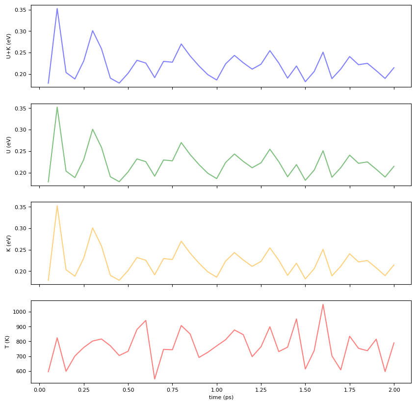
import pandas as pd

log_filename = output_filename + ".log"
df = pd.read_csv(log_filename, delim_whitespace=True, skiprows=1,
                 names=['Time[ps]','Etot/N[eV]','Epot/N[eV]','Ekin/N[eV]','T[K]','stress(xx)','stress(yy)','stress(zz)','stress(yz)','stress(xz)','stress(xy)'])
dfimport matplotlib.pyplot as plt
fig = plt.figure(figsize=(10, 10))
#color = 'tab:grey'
ax1 = fig.add_subplot(4, 1, 1)
ax1.set_xticklabels([])
ax1.set_ylabel('U+K (eV)')
ax1.plot(df["Time[ps]"], df["Etot/N[eV]"], color="blue",alpha=0.5)
ax2 = fig.add_subplot(4, 1, 2)
ax2.set_xticklabels([])
ax2.set_ylabel('U (eV)')
ax2.plot(df["Time[ps]"], df["Etot/N[eV]"], color="green",alpha=0.5)
ax3 = fig.add_subplot(4, 1, 3)
ax3.set_xticklabels([])
ax3.set_ylabel('K (eV)')
ax3.plot(df["Time[ps]"], df["Etot/N[eV]"], color="orange",alpha=0.5)
ax4 = fig.add_subplot(4, 1, 4)
ax4.set_xlabel('time (ps)')
ax4.set_ylabel('T (K)')
ax4.plot(df["Time[ps]"], df["T[K]"], color="red",alpha=0.5)
plt.show()
Data Splitting
We then need to devide the data into training/validation and test sets. The training set is used to train the MACE model, while the test set is used to evaluate its performance. We will use a 90-10 split for this example.
from ase.io import read, write
import random

atoms = read('./tmp/Cu_fcc_2x2x2.xyz', index=":", format='extxyz',parallel=True)
print(f"Number of data: {len(atoms)}")

# Randomly shuffle the data
seed = 123
random.seed(seed)

# determine the index to split an 90% / 10% data
split_idx = int(0.9 * len(atoms))
indices = list(range(len(atoms)))
random.shuffle(indices)

train_atoms = [atoms[i] for i in indices[:split_idx]]
test_atoms = [atoms[i] for i in indices[split_idx:]]

write("tmp/train_valid.xyz", train_atoms, format="extxyz")
write("tmp/test.xyz", test_atoms, format="extxyz")
Number of data: 40
Training Configuration
You can use the code below to generate training configuration. For more information, please refer to: https://
%%writefile ./tmp/training_config.yml

model: "MACE"
num_channels: 32
max_L: 0
r_max: 4.0
name: "mace01"
model_dir: "tmp/MACE_models"
log_dir: "tmp/MACE_models"
checkpoints_dir: "tmp/MACE_models"
results_dir: "tmp/MACE_models"
train_file: "tmp/train_valid.xyz"
valid_fraction: 0.10
test_file: "tmp/test.xyz"
energy_key: "energy"
forces_key: "forces"
stress_key: "stress"
E0s: "{29:3.5100}"
device: cpu
batch_size: 4
max_num_epochs: 50
swa: True
seed: 123
Overwriting ./tmp/training_config.yml
import warnings
warnings.filterwarnings("ignore")
from mace.cli.run_train import main as mace_run_train_main
import sys
import logging

def train_mace(config_file_path):
    logging.getLogger().handlers.clear()
    sys.argv = ["program", "--config", config_file_path]
    mace_run_train_main()
Training the MACE Model
Now we can start training the MACE model. This process might be time-consuming, depending on the size of your dataset and the complexity of the model. The training process involves optimizing the model parameters to minimize the difference between the predicted and target energies and forces.
train_mace("tmp/training_config.yml")2025-04-16 03:48:29.777 INFO: ===========VERIFYING SETTINGS===========
2025-04-16 03:48:29.778 INFO: MACE version: 0.3.12
2025-04-16 03:48:29.778 INFO: Using CPU
2025-04-16 03:48:29.849 INFO: ===========LOADING INPUT DATA===========
2025-04-16 03:48:29.850 INFO: Using heads: ['default']
2025-04-16 03:48:29.851 INFO: ============= Processing head default ===========
2025-04-16 03:48:29.867 WARNING: Since ASE version 3.23.0b1, using energy_key 'energy' is no longer safe when communicating between MACE and ASE. We recommend using a different key, rewriting 'energy' to 'REF_energy'. You need to use --energy_key='REF_energy' to specify the chosen key name.
2025-04-16 03:48:29.870 WARNING: Since ASE version 3.23.0b1, using forces_key 'forces' is no longer safe when communicating between MACE and ASE. We recommend using a different key, rewriting 'forces' to 'REF_forces'. You need to use --forces_key='REF_forces' to specify the chosen key name.
2025-04-16 03:48:29.873 WARNING: Since ASE version 3.23.0b1, using stress_key 'stress' is no longer safe when communicating between MACE and ASE. We recommend using a different key, rewriting 'stress' to 'REF_stress'. You need to use --stress_key='REF_stress' to specify the chosen key name.
2025-04-16 03:48:29.877 INFO: Training file 1/1 [36 configs, 36 energy, 36 forces, 36 stresses] loaded from 'tmp/train_valid.xyz'
2025-04-16 03:48:29.878 INFO: Total training set [36 configs, 36 energy, 36 forces, 36 stresses]
2025-04-16 03:48:29.878 INFO: Using random 10% of training set for validation with following indices: [27, 25, 13]
2025-04-16 03:48:29.879 INFO: Validation set contains 3 configurations [3 energy, 3 forces, 3 stresses]
2025-04-16 03:48:29.884 WARNING: Since ASE version 3.23.0b1, using energy_key 'energy' is no longer safe when communicating between MACE and ASE. We recommend using a different key, rewriting 'energy' to 'REF_energy'. You need to use --energy_key='REF_energy' to specify the chosen key name.
2025-04-16 03:48:29.885 WARNING: Since ASE version 3.23.0b1, using forces_key 'forces' is no longer safe when communicating between MACE and ASE. We recommend using a different key, rewriting 'forces' to 'REF_forces'. You need to use --forces_key='REF_forces' to specify the chosen key name.
2025-04-16 03:48:29.886 WARNING: Since ASE version 3.23.0b1, using stress_key 'stress' is no longer safe when communicating between MACE and ASE. We recommend using a different key, rewriting 'stress' to 'REF_stress'. You need to use --stress_key='REF_stress' to specify the chosen key name.
2025-04-16 03:48:29.887 INFO: Test file 1/1 [4 configs, 4 energy, 4 forces, 4 stresses] loaded from 'tmp/test.xyz'
2025-04-16 03:48:29.888 INFO: Total test set (4 configs):
2025-04-16 03:48:29.888 INFO: Default_default: 4 configs, 4 energy, 4 forces, 4 stresses
2025-04-16 03:48:29.889 INFO: Total number of configurations: train=33, valid=3, tests=[Default_default: 4],
2025-04-16 03:48:29.893 WARNING: Validation batch size (10) is larger than the number of validation data (3)
2025-04-16 03:48:29.893 INFO: Atomic Numbers used: [29]
2025-04-16 03:48:29.894 INFO: Isolated Atomic Energies (E0s) not in training file, using command line argument
2025-04-16 03:48:29.895 INFO: Atomic Energies used (z: eV) for head default: {29: 3.51}
2025-04-16 03:48:29.895 INFO: Processing datasets for head 'default'
2025-04-16 03:48:29.962 INFO: Combining 1 list datasets for head 'default'
2025-04-16 03:48:29.965 INFO: Head 'default' training dataset size: 33
2025-04-16 03:48:29.966 INFO: Computing average number of neighbors
2025-04-16 03:48:29.973 INFO: Average number of neighbors: 17.7578125
2025-04-16 03:48:29.973 INFO: During training the following quantities will be reported: energy, forces
2025-04-16 03:48:29.974 INFO: ===========MODEL DETAILS===========
2025-04-16 03:48:29.980 INFO: Building model
2025-04-16 03:48:29.981 INFO: Message passing with 32 channels and max_L=0 (32x0e)
2025-04-16 03:48:29.982 INFO: 2 layers, each with correlation order: 3 (body order: 4) and spherical harmonics up to: l=3
2025-04-16 03:48:29.982 INFO: 8 radial and 5 basis functions
2025-04-16 03:48:29.983 INFO: Radial cutoff: 4.0 A (total receptive field for each atom: 8.0 A)
2025-04-16 03:48:29.984 INFO: Distance transform for radial basis functions: None
2025-04-16 03:48:29.985 INFO: Hidden irreps: 32x0e
2025-04-16 03:48:30.543 INFO: Total number of parameters: 53584
2025-04-16 03:48:30.543 INFO:
2025-04-16 03:48:30.544 INFO: ===========OPTIMIZER INFORMATION===========
2025-04-16 03:48:30.545 INFO: Using ADAM as parameter optimizer
2025-04-16 03:48:30.545 INFO: Batch size: 4
2025-04-16 03:48:30.545 INFO: Number of gradient updates: 412
2025-04-16 03:48:30.546 INFO: Learning rate: 0.01, weight decay: 5e-07
2025-04-16 03:48:30.546 INFO: WeightedEnergyForcesLoss(energy_weight=1.000, forces_weight=100.000)
2025-04-16 03:48:30.547 INFO: Stage Two (after 36 epochs) with loss function: WeightedEnergyForcesLoss(energy_weight=1000.000, forces_weight=100.000), with energy weight : 1000.0, forces weight : 100.0 and learning rate : 0.001
2025-04-16 03:48:30.598 INFO: Using gradient clipping with tolerance=10.000
2025-04-16 03:48:30.599 INFO:
2025-04-16 03:48:30.599 INFO: ===========TRAINING===========
2025-04-16 03:48:30.600 INFO: Started training, reporting errors on validation set
2025-04-16 03:48:30.600 INFO: Loss metrics on validation set
2025-04-16 03:48:30.679 INFO: Initial: head: default, loss=19.75021945, RMSE_E_per_atom= 3442.74 meV, RMSE_F= 688.46 meV / A
2025-04-16 03:48:31.930 INFO: Epoch 0: head: default, loss=12.65267467, RMSE_E_per_atom= 3028.92 meV, RMSE_F= 536.50 meV / A
2025-04-16 03:48:33.177 INFO: Epoch 1: head: default, loss=5.00620433, RMSE_E_per_atom= 3025.40 meV, RMSE_F= 242.19 meV / A
2025-04-16 03:48:34.440 INFO: Epoch 2: head: default, loss=4.23638255, RMSE_E_per_atom= 2685.92 meV, RMSE_F= 234.41 meV / A
2025-04-16 03:48:35.765 INFO: Epoch 3: head: default, loss=2.51651391, RMSE_E_per_atom= 2548.65 meV, RMSE_F= 102.66 meV / A
2025-04-16 03:48:36.994 INFO: Epoch 4: head: default, loss=1.67258795, RMSE_E_per_atom= 2071.25 meV, RMSE_F= 85.30 meV / A
2025-04-16 03:48:38.207 INFO: Epoch 5: head: default, loss=0.65792243, RMSE_E_per_atom= 1117.16 meV, RMSE_F= 85.19 meV / A
2025-04-16 03:48:39.770 INFO: Epoch 6: head: default, loss=0.25720635, RMSE_E_per_atom= 186.23 meV, RMSE_F= 85.85 meV / A
2025-04-16 03:48:41.167 INFO: Epoch 7: head: default, loss=0.17780661, RMSE_E_per_atom= 66.33 meV, RMSE_F= 72.73 meV / A
2025-04-16 03:48:42.440 INFO: Epoch 8: head: default, loss=0.11830597, RMSE_E_per_atom= 55.59 meV, RMSE_F= 59.32 meV / A
2025-04-16 03:48:43.671 INFO: Epoch 9: head: default, loss=0.12779799, RMSE_E_per_atom= 217.82 meV, RMSE_F= 57.96 meV / A
2025-04-16 03:48:44.965 INFO: Epoch 10: head: default, loss=0.27851048, RMSE_E_per_atom= 47.46 meV, RMSE_F= 91.28 meV / A
2025-04-16 03:48:46.292 INFO: Epoch 11: head: default, loss=0.33426494, RMSE_E_per_atom= 56.11 meV, RMSE_F= 99.98 meV / A
2025-04-16 03:48:47.530 INFO: Epoch 12: head: default, loss=0.07611942, RMSE_E_per_atom= 17.80 meV, RMSE_F= 47.75 meV / A
2025-04-16 03:48:48.866 INFO: Epoch 13: head: default, loss=0.04599848, RMSE_E_per_atom= 23.20 meV, RMSE_F= 37.08 meV / A
2025-04-16 03:48:50.237 INFO: Epoch 14: head: default, loss=0.07709748, RMSE_E_per_atom= 22.26 meV, RMSE_F= 48.04 meV / A
2025-04-16 03:48:51.480 INFO: Epoch 15: head: default, loss=0.04451550, RMSE_E_per_atom= 29.31 meV, RMSE_F= 36.43 meV / A
2025-04-16 03:48:52.661 INFO: Epoch 16: head: default, loss=0.04861449, RMSE_E_per_atom= 27.74 meV, RMSE_F= 38.09 meV / A
2025-04-16 03:48:53.987 INFO: Epoch 17: head: default, loss=0.02026954, RMSE_E_per_atom= 19.63 meV, RMSE_F= 24.58 meV / A
2025-04-16 03:48:55.292 INFO: Epoch 18: head: default, loss=0.03726097, RMSE_E_per_atom= 12.09 meV, RMSE_F= 33.41 meV / A
2025-04-16 03:48:56.542 INFO: Epoch 19: head: default, loss=0.01654074, RMSE_E_per_atom= 12.63 meV, RMSE_F= 22.24 meV / A
2025-04-16 03:48:57.976 INFO: Epoch 20: head: default, loss=0.01975056, RMSE_E_per_atom= 13.87 meV, RMSE_F= 24.30 meV / A
2025-04-16 03:48:59.240 INFO: Epoch 21: head: default, loss=0.01652776, RMSE_E_per_atom= 32.27 meV, RMSE_F= 22.03 meV / A
2025-04-16 03:49:00.471 INFO: Epoch 22: head: default, loss=0.02347430, RMSE_E_per_atom= 15.22 meV, RMSE_F= 26.49 meV / A
2025-04-16 03:49:01.817 INFO: Epoch 23: head: default, loss=0.01546703, RMSE_E_per_atom= 11.17 meV, RMSE_F= 21.51 meV / A
2025-04-16 03:49:03.165 INFO: Epoch 24: head: default, loss=0.01725255, RMSE_E_per_atom= 11.34 meV, RMSE_F= 22.72 meV / A
2025-04-16 03:49:04.426 INFO: Epoch 25: head: default, loss=0.02783829, RMSE_E_per_atom= 38.14 meV, RMSE_F= 28.65 meV / A
2025-04-16 03:49:05.731 INFO: Epoch 26: head: default, loss=0.01551675, RMSE_E_per_atom= 19.86 meV, RMSE_F= 21.48 meV / A
2025-04-16 03:49:07.050 INFO: Epoch 27: head: default, loss=0.01771259, RMSE_E_per_atom= 12.89 meV, RMSE_F= 23.02 meV / A
2025-04-16 03:49:08.344 INFO: Epoch 28: head: default, loss=0.03725313, RMSE_E_per_atom= 20.50 meV, RMSE_F= 33.37 meV / A
2025-04-16 03:49:09.670 INFO: Epoch 29: head: default, loss=0.02399820, RMSE_E_per_atom= 19.13 meV, RMSE_F= 26.76 meV / A
2025-04-16 03:49:10.906 INFO: Epoch 30: head: default, loss=0.02265691, RMSE_E_per_atom= 15.35 meV, RMSE_F= 26.03 meV / A
2025-04-16 03:49:12.081 INFO: Epoch 31: head: default, loss=0.01256153, RMSE_E_per_atom= 33.81 meV, RMSE_F= 19.12 meV / A
2025-04-16 03:49:13.292 INFO: Epoch 32: head: default, loss=0.01721157, RMSE_E_per_atom= 16.74 meV, RMSE_F= 22.66 meV / A
2025-04-16 03:49:14.512 INFO: Epoch 33: head: default, loss=0.01854147, RMSE_E_per_atom= 10.98 meV, RMSE_F= 23.56 meV / A
2025-04-16 03:49:15.727 INFO: Epoch 34: head: default, loss=0.01330458, RMSE_E_per_atom= 12.42 meV, RMSE_F= 19.94 meV / A
2025-04-16 03:49:16.863 INFO: Epoch 35: head: default, loss=0.01104176, RMSE_E_per_atom= 13.66 meV, RMSE_F= 18.15 meV / A
2025-04-16 03:49:16.900 INFO: Changing loss based on Stage Two Weights
2025-04-16 03:49:18.063 INFO: Epoch 36: head: default, loss=1.18592731, RMSE_E_per_atom= 59.14 meV, RMSE_F= 24.46 meV / A
2025-04-16 03:49:19.278 INFO: Epoch 37: head: default, loss=0.53699927, RMSE_E_per_atom= 39.03 meV, RMSE_F= 29.66 meV / A
2025-04-16 03:49:20.473 INFO: Epoch 38: head: default, loss=0.24354356, RMSE_E_per_atom= 24.81 meV, RMSE_F= 33.96 meV / A
2025-04-16 03:49:21.677 INFO: Epoch 39: head: default, loss=0.16964108, RMSE_E_per_atom= 19.63 meV, RMSE_F= 35.17 meV / A
2025-04-16 03:49:22.914 INFO: Epoch 40: head: default, loss=0.26512949, RMSE_E_per_atom= 26.78 meV, RMSE_F= 27.96 meV / A
2025-04-16 03:49:24.087 INFO: Epoch 41: head: default, loss=0.05382714, RMSE_E_per_atom= 9.79 meV, RMSE_F= 25.61 meV / A
2025-04-16 03:49:25.337 INFO: Epoch 42: head: default, loss=0.25393172, RMSE_E_per_atom= 26.37 meV, RMSE_F= 25.81 meV / A
2025-04-16 03:49:26.576 INFO: Epoch 43: head: default, loss=0.04461799, RMSE_E_per_atom= 8.90 meV, RMSE_F= 23.38 meV / A
2025-04-16 03:49:27.788 INFO: Epoch 44: head: default, loss=0.05101512, RMSE_E_per_atom= 9.99 meV, RMSE_F= 23.09 meV / A
2025-04-16 03:49:28.966 INFO: Epoch 45: head: default, loss=0.14435939, RMSE_E_per_atom= 19.17 meV, RMSE_F= 25.59 meV / A
2025-04-16 03:49:30.173 INFO: Epoch 46: head: default, loss=0.04314693, RMSE_E_per_atom= 8.42 meV, RMSE_F= 24.21 meV / A
2025-04-16 03:49:31.368 INFO: Epoch 47: head: default, loss=0.03901319, RMSE_E_per_atom= 8.24 meV, RMSE_F= 22.19 meV / A
2025-04-16 03:49:32.550 INFO: Epoch 48: head: default, loss=0.06649804, RMSE_E_per_atom= 12.37 meV, RMSE_F= 21.54 meV / A
2025-04-16 03:49:33.689 INFO: Epoch 49: head: default, loss=0.04361523, RMSE_E_per_atom= 8.92 meV, RMSE_F= 22.63 meV / A
2025-04-16 03:49:33.690 INFO: Training complete
2025-04-16 03:49:33.690 INFO:
2025-04-16 03:49:33.690 INFO: ===========RESULTS===========
2025-04-16 03:49:33.695 INFO: Loading checkpoint: tmp/MACE_models/mace01_run-123_epoch-35.pt
2025-04-16 03:49:33.712 INFO: Loaded Stage one model from epoch 35 for evaluation
2025-04-16 03:49:33.714 INFO: Saving model to tmp/MACE_models/mace01_run-123.model
2025-04-16 03:49:33.825 INFO: Compiling model, saving metadata to tmp/MACE_models/mace01_compiled.model
2025-04-16 03:49:34.153 INFO: Computing metrics for training, validation, and test sets
2025-04-16 03:49:34.154 INFO: Evaluating train_default ...
2025-04-16 03:49:34.706 INFO: Evaluating valid_default ...
2025-04-16 03:49:34.763 INFO: Error-table on TRAIN and VALID:
+---------------+---------------------+------------------+-------------------+
| config_type | RMSE E / meV / atom | RMSE F / meV / A | relative F RMSE % |
+---------------+---------------------+------------------+-------------------+
| train_default | 29.2 | 19.5 | 2.73 |
| valid_default | 13.7 | 18.1 | 2.65 |
+---------------+---------------------+------------------+-------------------+
2025-04-16 03:49:34.763 INFO: Evaluating Default_default ...
2025-04-16 03:49:34.837 INFO: Error-table on TEST:
+-----------------+---------------------+------------------+-------------------+
| config_type | RMSE E / meV / atom | RMSE F / meV / A | relative F RMSE % |
+-----------------+---------------------+------------------+-------------------+
| Default_default | 42.4 | 20.1 | 2.86 |
+-----------------+---------------------+------------------+-------------------+
2025-04-16 03:49:36.270 INFO: Loading checkpoint: tmp/MACE_models/mace01_run-123_epoch-47_swa.pt
2025-04-16 03:49:36.275 INFO: Loaded Stage two model from epoch 47 for evaluation
2025-04-16 03:49:36.276 INFO: Saving model to tmp/MACE_models/mace01_run-123_stagetwo.model
2025-04-16 03:49:36.405 INFO: Compiling model, saving metadata tmp/MACE_models/mace01_stagetwo_compiled.model
2025-04-16 03:49:36.755 INFO: Computing metrics for training, validation, and test sets
2025-04-16 03:49:36.756 INFO: Evaluating train_default ...
2025-04-16 03:49:37.184 INFO: Evaluating valid_default ...
2025-04-16 03:49:37.230 INFO: Error-table on TRAIN and VALID:
+---------------+---------------------+------------------+-------------------+
| config_type | RMSE E / meV / atom | RMSE F / meV / A | relative F RMSE % |
+---------------+---------------------+------------------+-------------------+
| train_default | 6.7 | 26.9 | 3.78 |
| valid_default | 8.2 | 22.2 | 3.24 |
+---------------+---------------------+------------------+-------------------+
2025-04-16 03:49:37.230 INFO: Evaluating Default_default ...
2025-04-16 03:49:37.280 INFO: Error-table on TEST:
+-----------------+---------------------+------------------+-------------------+
| config_type | RMSE E / meV / atom | RMSE F / meV / A | relative F RMSE % |
+-----------------+---------------------+------------------+-------------------+
| Default_default | 5.3 | 27.6 | 3.93 |
+-----------------+---------------------+------------------+-------------------+
2025-04-16 03:49:38.376 INFO: Done
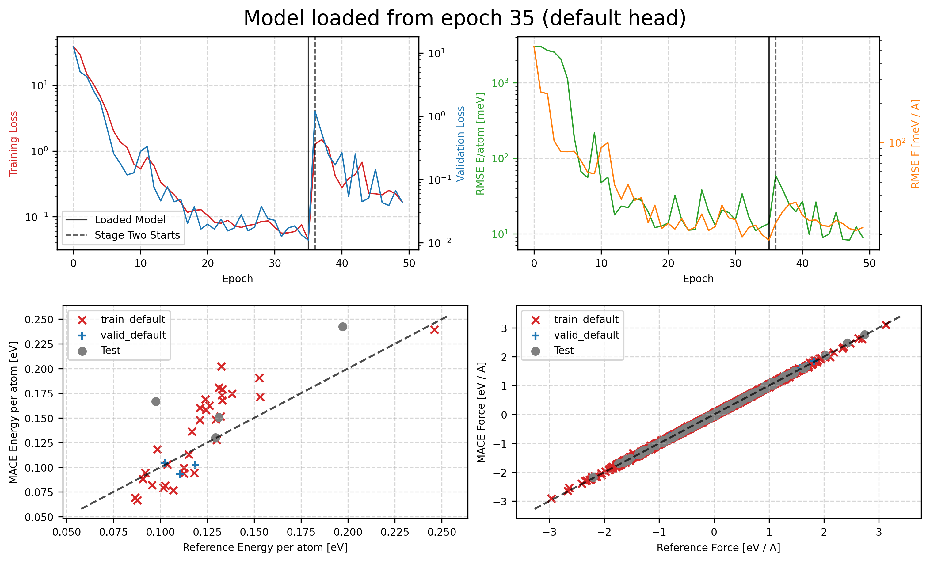
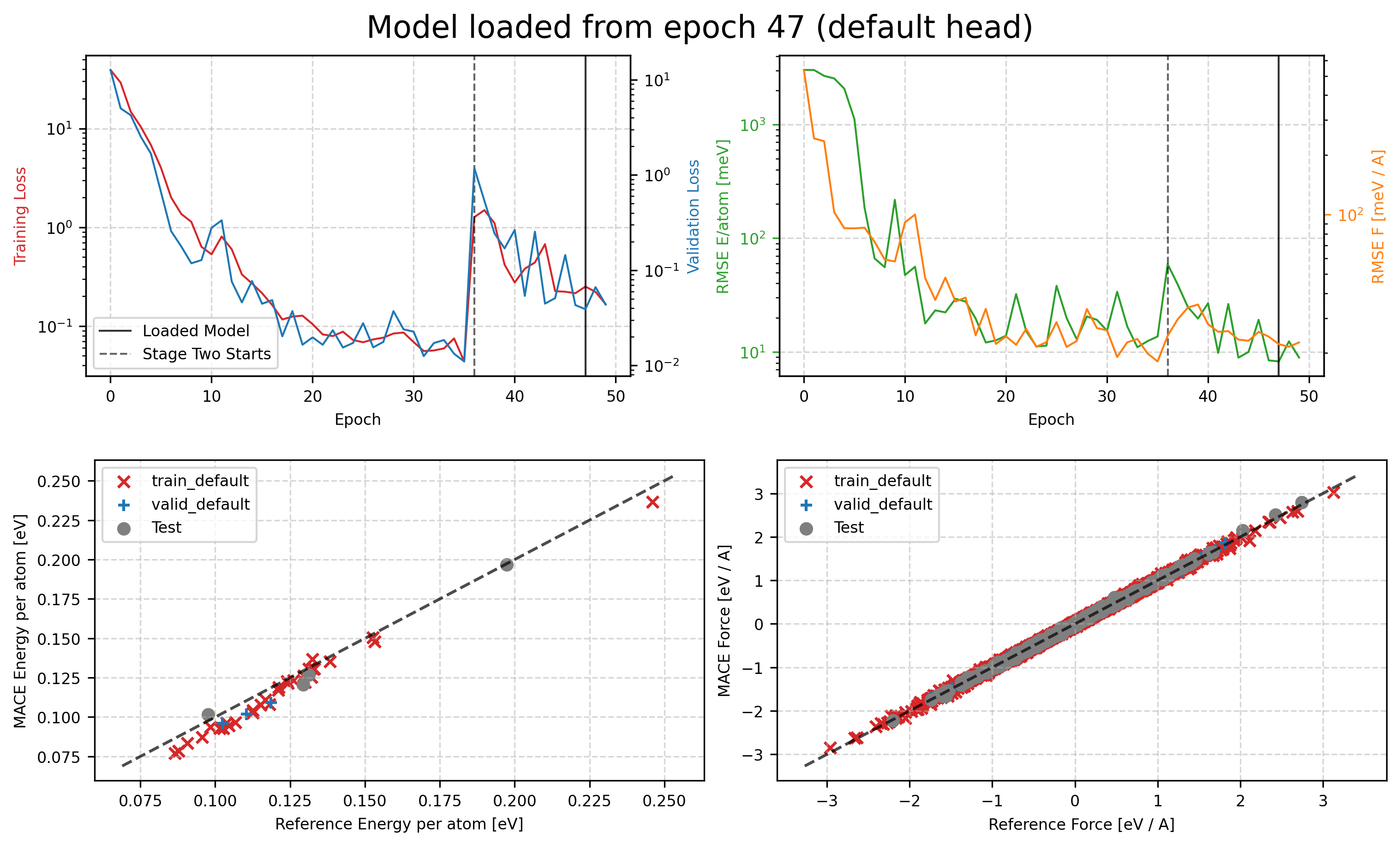
Track Training Results
You can then check the training curves in tmp/MACE_models/mace01_run-123_train_default_stage_one.png and tmp/MACE_models/mace01_run-123_train_default_stage_two.png to see how the training process goes. The first one is the training curve for stage one, and the second one is for stage two.
from IPython.display import Image, display

display(Image(filename='tmp/MACE_models/mace01_run-123_train_default_stage_one.png'))
display(Image(filename='tmp/MACE_models/mace01_run-123_train_default_stage_two.png'))
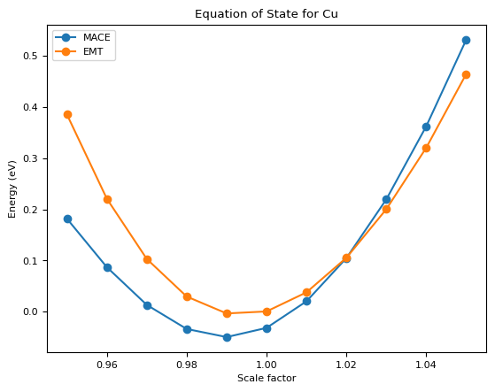
Further Test: Equation of State
Then we can test the equation of state of the model.
from mace.calculators import MACECalculator
import numpy as np
from ase.eos import EquationOfState
calculator = MACECalculator(
    model_paths="tmp/MACE_models/mace01_run-123_stagetwo.model",
    device="cpu")

import matplotlib.pyplot as plt
# Define a range of scale factors
scale_factors = np.linspace(0.95, 1.05, 11)
energies_mace = []
energies_emt = []
volumes = []
atoms = bulk("Cu", "fcc", cubic=True, a=3.615)
atoms.pbc = True

for s in scale_factors:
    # Make a copy of the original bulk Cu structure
    atoms_scaled = atoms.copy()

    # Scale the cell and positions accordingly
    atoms_scaled.set_cell(atoms_scaled.get_cell() * s, scale_atoms=True)

    atoms_scaled_emt = atoms_scaled.copy()
    # Assign the MACE calculator
    atoms_scaled.calc = calculator

    atoms_scaled_emt.calc = EMT()
    volumes.append(atoms_scaled.get_volume())
    # Compute and store the potential energy
    energies_mace.append(atoms_scaled.get_potential_energy())
    energies_emt.append(atoms_scaled_emt.get_potential_energy())

eos_mace = EquationOfState(volumes, energies_mace)
eos_emt = EquationOfState(volumes, energies_emt)

# Fit the EOS to the MACE energies
v0_mace, e0_mace, B_mace = eos_mace.fit()
# Fit the EOS to the EMT energies
v0_emt, e0_emt, B_emt = eos_emt.fit()

print(f"MACE: v0 = {v0_mace:.4f}, e0 = {e0_mace:.4f}, B = {B_mace:.4f}")
print(f"EMT: v0 = {v0_emt:.4f}, e0 = {e0_emt:.4f}, B = {B_emt:.4f}")

# Plot the Equation of State (EOS)
plt.figure()
plt.plot(scale_factors, energies_mace, marker="o", label="MACE")
plt.plot(scale_factors, energies_emt, marker="o", label="EMT")
plt.legend()
plt.xlabel("Scale factor")
plt.ylabel("Energy (eV)")
plt.title("Equation of State for Cu")
plt.show()
2025-04-16 03:50:10.278 INFO: Using CPU
No dtype selected, switching to float64 to match model dtype.
MACE: v0 = 45.7100, e0 = -0.0468, B = 0.7390
EMT: v0 = 46.3859, e0 = -0.0062, B = 0.8378