Why MLPs?
Machine learning potentials (MLPs) are a class of interatomic potentials that use machine learning techniques to predict the potential energy surface (PES) of a system. The forces and stresses are available through analytical derivatives of the energy. They are designed to provide accurate and efficient approximations of the potential energy and forces acting on atoms in a material, making them suitable for large-scale molecular dynamics simulations.
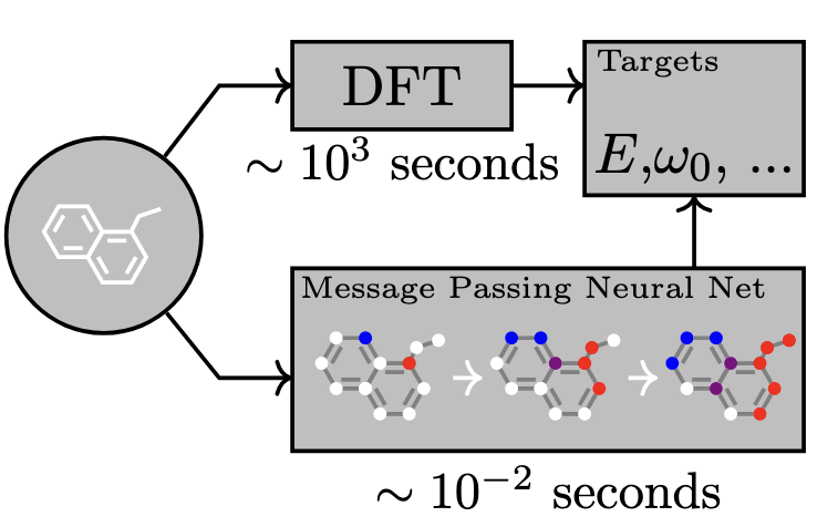
A message passing neural network (MPNN) can predict the energy and properties of a system using a fraction of the time compared to DFT. Figure adapted from Gilmer et al. (2017)
There are two category of interatomic potentials: physics-based potentials (PBPs) and first-principles. PBPs, or classical force fields, are based on physical models and parameters that are fitted to experimental data or high-level quantum mechanical calculations. They are computationally efficient but may not accurately capture the complex interactions in some systems. First-principles methods, such as density functional theory (DFT), provide highly accurate results but are computationally expensive and not suitable for large systems or long time scales.
| Classical force fields | Quantum mechanical methods | Machine learning potentials | |
|---|---|---|---|
| Model complexity | Simple analytical model | Quantum mechanical model | Machine learning model |
| Model building | Hard, need to understand deeply for each material | Very easy, no need to build force field | Medium, need to collect data and train the model |
| Speed and cost | Very fast and very cheap to compute (106 to 107 atoms in nano-seconds) | Slow and expensive: 102 to 103 atoms in 102 pico-seconds | Fast and cheap: 103 to 104 atoms in nano-seconds |
| Transferability | Poor, need to build potential for each system | Good, can be used for most systems, even for unknown system | Depends on your dataset |
| Accuracy | Tens to hundred of meV/atom | 1-2 meV/atom | A few to tens of meV/atom |
MLPs bridge the gap between these two approaches by using machine learning techniques to learn the potential energy surface from a set of reference data, which can be obtained from first-principles calculations. This allows MLPs to achieve high accuracy while maintaining computational efficiency.
Compared to PGPs, MLPs utilize a variety of machine learning techniques, including neural networks, Gaussian processes, kernel ridge regression, and others to model the potential energy surface. MLPs are more flexible and can capture complex interactions between atoms, making them suitable for a wide range of materials and systems. It is much easier to develop MLP for a new material than to develop a new PBP because PBP needs lots of domain knowledge and experience whereas MLPs can be trained on a dataset of atomic configurations and their corresponding energies, forces, and stresses. MLPs can also be improved iteratively by adding more training data, which is not that easy with traditional PBPs. The training process of MLPs is generally easy and straightforward using existing software packages such as PyTorch, which we have used in the previous lectures.
However, a reliable and universal MLP needs to be trained on a large dataset of atomic configurations and their corresponding DFT energies, forces and stresses.
Formalism
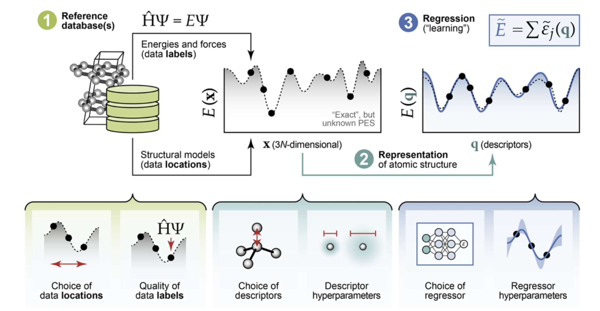
The general process of making a MLP. Figure adapted from Morrow et al. (2023)
The basic idea of MLPs is to approximate the Born-Oppenheimer Potential Energy Surface (PES). This surface describes the potential energy of a system as a function of the positions of all its aotmic nuclei.
where is the total energy of the system, and is the position of the -th atom.
The forces are simply the negative graidient of the energy with respect to the atomic positions:
The positions of the atomic nuclei are converted to a feature vector. Then this feature vector will be fed into a ML model.
There are two types of features: explicit and implicit features. We will introduce them in the following sections.
- Gilmer, J., Schoenholz, S. S., Riley, P. F., Vinyals, O., & Dahl, G. E. (2017). Neural Message Passing for Quantum Chemistry. arXiv. 10.48550/ARXIV.1704.01212
- Morrow, J. D., Gardner, J. L. A., & Deringer, V. L. (2023). How to validate machine-learned interatomic potentials. The Journal of Chemical Physics, 158(12). 10.1063/5.0139611