Local Optimization
These methods are good at finding local minima. They are often used when you have a reasonable starting point or when the objective function is relatively smooth (ideally, convex).
Line Search
Line search is a method for finding the minimum of a function along a given direction. It’s often used in conjunction with other optimization methods that require a search direction (e.g., gradient descent, Newton’s method). An example of a line search algorithm is the golden section search.
Golden section search is a method for finding the minimum (or maximum) of a unimodal function within a specified interval. It is a derivative-free optimization technique that relies on the golden ratio to reduce the search interval at each step.
Algorithm
Define the interval where the minimum lies.
Compute two interior points:
where is the golden ratio.
Evaluate the function at and .
Narrow the interval:
If , the new interval is .
Otherwise, the new interval is .
Repeat steps 2-4 until the interval is sufficiently small.
The minimum is approximately at the midpoint of the final interval.
Advantages and Disadvantages
Does not require derivatives, making it suitable for non-differentiable or noisy functions.
Efficient for unimodal functions due to the constant reduction factor provided by the golden ratio.
Only works for unimodal functions within the specified interval.
Slower convergence compared to methods that use gradient information.
Golden section search is often used in line search procedures within larger optimization algorithms.
Gradient Descent
This is the workhorse of many optimization problems. It works by iteratively taking steps in the direction of the negative gradient.
The algorithm is simple:
Choose an initial guess, .
Calculate the gradient, , at the current point.
Update the position: , where is the learning rate (a small positive number that controls the step size).
Repeat steps 2 and 3 until a convergence criterion is met (e.g., the gradient becomes very small, or the change in the objective function is negligible).
Learning Rate () should be chosen properly: If is too small, the convergence will be very slow. If is too large, the algorithm might overshoot the minimum and oscillate or even diverge. There are various strategies for choosing and adapting the learning rate (e.g., using a fixed value, decreasing it over time, or using more sophisticated methods like Adam).
GD is simple to implement but can be slow for high-dimensional problems or functions with many local minima and is sensitive to the choice of learning rate.
Variants: Stochastic Gradient Descent (SGD, for large datasets, updates with a subset of the data), Momentum (adds a “momentum” term to accelerate convergence and escape shallow local minima), Adam (combines momentum and adaptive learning rates).
Conjugate Gradient
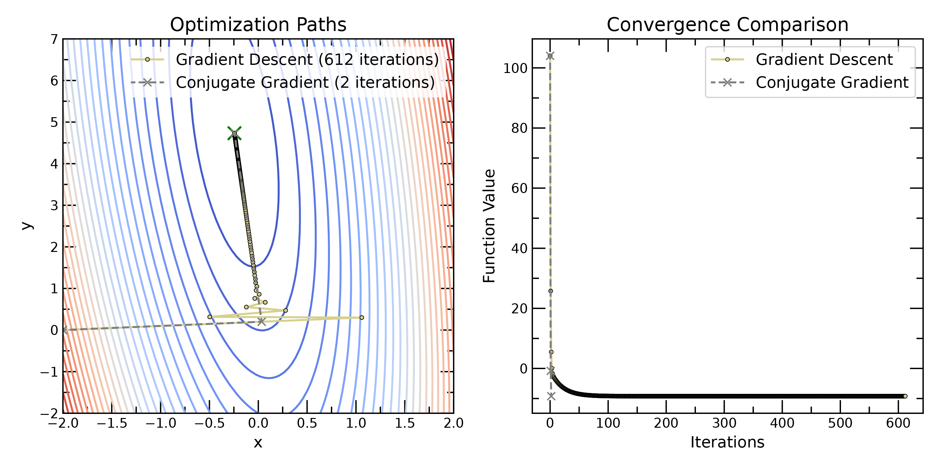
Comparison of gradient descent and conjugate gradient methods. Conjugate gradient methods can converge more quickly than gradient descent, especially for quadratic functions.
Gradient descent can sometimes “zig-zag” inefficiently, especially in valleys with steep sides. Conjugate gradient methods improve upon this by choosing search directions that are conjugate to each other. This ensures that each step makes progress in a new, independent direction. CG converges more quickly than GD for many problems, particularly when the objective function is quadratic.
The search direction, , is calculated as:
where is a scalar that ensures conjugacy. Different formulas for exist (e.g., Fletcher-Reeves, Polak-Ribière). The key idea is that is a linear combination of the current negative gradient and the previous search direction. The update rule is then:
where is again chosen (often via line search) to minimize the function along the search direction.
Key Idea: Instead of just using the negative gradient, the search direction is a linear combination of the negative gradient and the previous search direction.
Newton’s Method
Newton’s method uses both the gradient and the Hessian matrix (second derivatives) to find the minimum of a function. It’s based on approximating the function locally by a quadratic function and then finding the minimum of that quadratic.
We want to find a point where the gradient is zero, . This is a necessary condition for a minimum (assuming the function is differentiable). Newton’s method uses a Taylor series expansion of the gradient around the current point, :
where is the Hessian matrix at . We want to find such that . Setting the right-hand side to zero and solving for , we get:
Algorithm:
Choose an initial guess, .
Calculate the gradient, , and the Hessian, , at the current point.
Calculate the update step: .
Update the position: .
Repeat steps 2-4 until a convergence criterion is met.
Near a minimum, Newton’s method converges very rapidly (much faster than gradient descent). The number of correct digits roughly doubles with each iteration. However, the Hessian can be computationally expensive to calculate, and the method can be sensitive to the choice of starting point. In addition, the Hessian must be nonsingular for the Newton step to be defined, and it should be positive definite if we want the step to be a local descent direction toward a minimum. If the Hessian is not positive definite, the method may diverge or move toward a saddle point or maximum.
BFGS (Broyden-Fletcher-Goldfarb-Shanno)
BFGS is a quasi-Newton method. Newton’s method uses the Hessian (matrix of second derivatives) to find the optimum. However, calculating the Hessian can be computationally expensive. BFGS approximates the Hessian iteratively, making it more practical for many problems.
BFGS iteratively updates an approximation to the inverse Hessian, denoted as . The update rule uses the change in the gradient and the change in the position to improve the approximation:
where
The search direction is then calculated as:
And the position update is:
(Again, is often found via line search.)
Key Idea: BFGS builds up an approximation to the inverse Hessian matrix over iterations, using gradient information. This approximation is used to determine the search direction. It is often more efficient than plain gradient descent for smooth problems.
Limited-memory BFGS (L-BFGS): For very high-dimensional problems (many variables), storing the full (approximate) Hessian in BFGS can become memory-intensive. L-BFGS stores only a limited number of past gradient and position updates, reducing memory requirements.
Other Local Optimization Methods
Nelder-Mead (Simplex) method doesn’t require derivatives. It constructs a simplex (a shape with vertices in dimensions) around the current point and iteratively shrinks, expands, or reflects the simplex to find the minimum.
Powell’s method is another derivative-free method that uses conjugate directions to find the minimum. It’s often more efficient than Nelder-Mead for high-dimensional problems.