Global Optimization
Local optimization methods can get trapped in local minima. Global optimization algorithms are designed to explore the search space more broadly, increasing the chances of finding the global optimum.
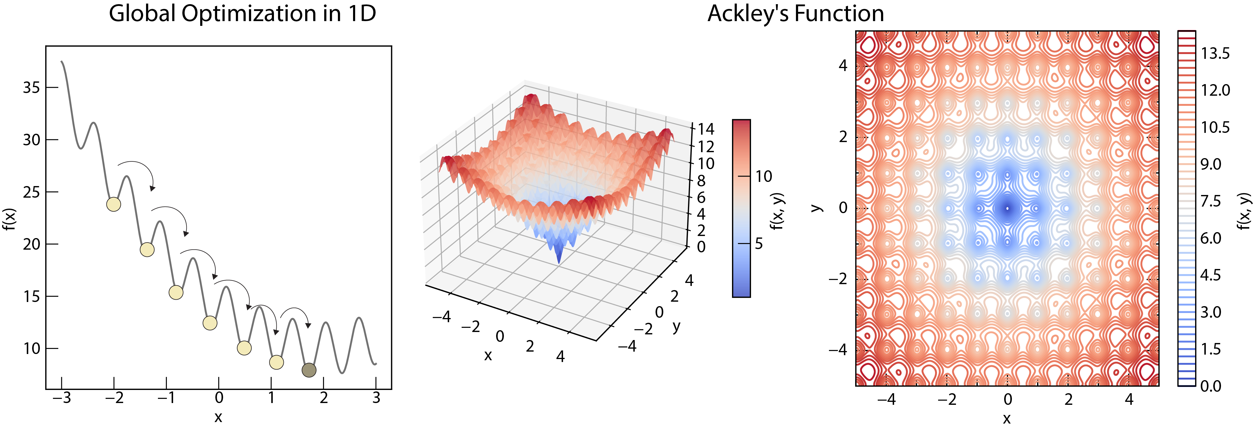
Global optimization aims to find the global minimum of a function, which may have multiple local minima. The example shows an Ackley function with multiple local minima and a single global minimum.
Simulated Annealing
Simulated annealing is inspired by the annealing process in metallurgy. Starts at a high “temperature” (allowing exploration) and gradually cools down (focusing on exploitation). Accepts moves that worsen the objective function with a probability that decreases with temperature.
Algorithm
Initialization: Start with an initial solution, , and a high “temperature,” .
Generate Neighbor: Generate a random neighboring solution, , by perturbing the current solution. The nature of the perturbation depends on the problem (e.g., for a continuous variable, you might add a random number drawnfrom a normal distribution; for a discrete variable, you might randomly changeone of the components).
Evaluate Energy Change: Calculate the change in the objective function (often referred to as “energy” in the context of simulated annealing), .
Acceptance Criterion:
If (the new solution is better), accept the new solution: .
If (the new solution is worse), accept the new solution with a probability given by the Metropolis criterion:
where is Boltzmann’s constant (often set to 1 in optimization contexts). It controls the probability of accepting worse solutions. High temperature allows for more exploration (escaping local minima), while low temperature favors exploitation (refining the solution near a good minimum). The prabablistic process ensures that the algorithm doesn’t get stuck in a local minimum too early.
Cooling: Reduce the temperature, , according to a cooling schedule. Common schedules include:
Linear Cooling: , where is a constant cooling rate.
Geometric Cooling: , where is a constant factor (typically between 0.8 and 0.99).
Adaptive Cooling: The cooling rate is adjusted based on the progress of the algorithm.
Cooling rate is crucial for the success of simulated annealing. Cooling too quickly can lead to premature convergence to a local minimum, while cooling too slowly is computationally inefficient.
Iteration: Repeat steps 2-5 until a stopping criterion is met (e.g., the temperature reaches a predefined minimum value, a maximum number of iterations is reached, or the objective function value hasn’t improved significantly for a certain number of iterations).
Basin Hopping
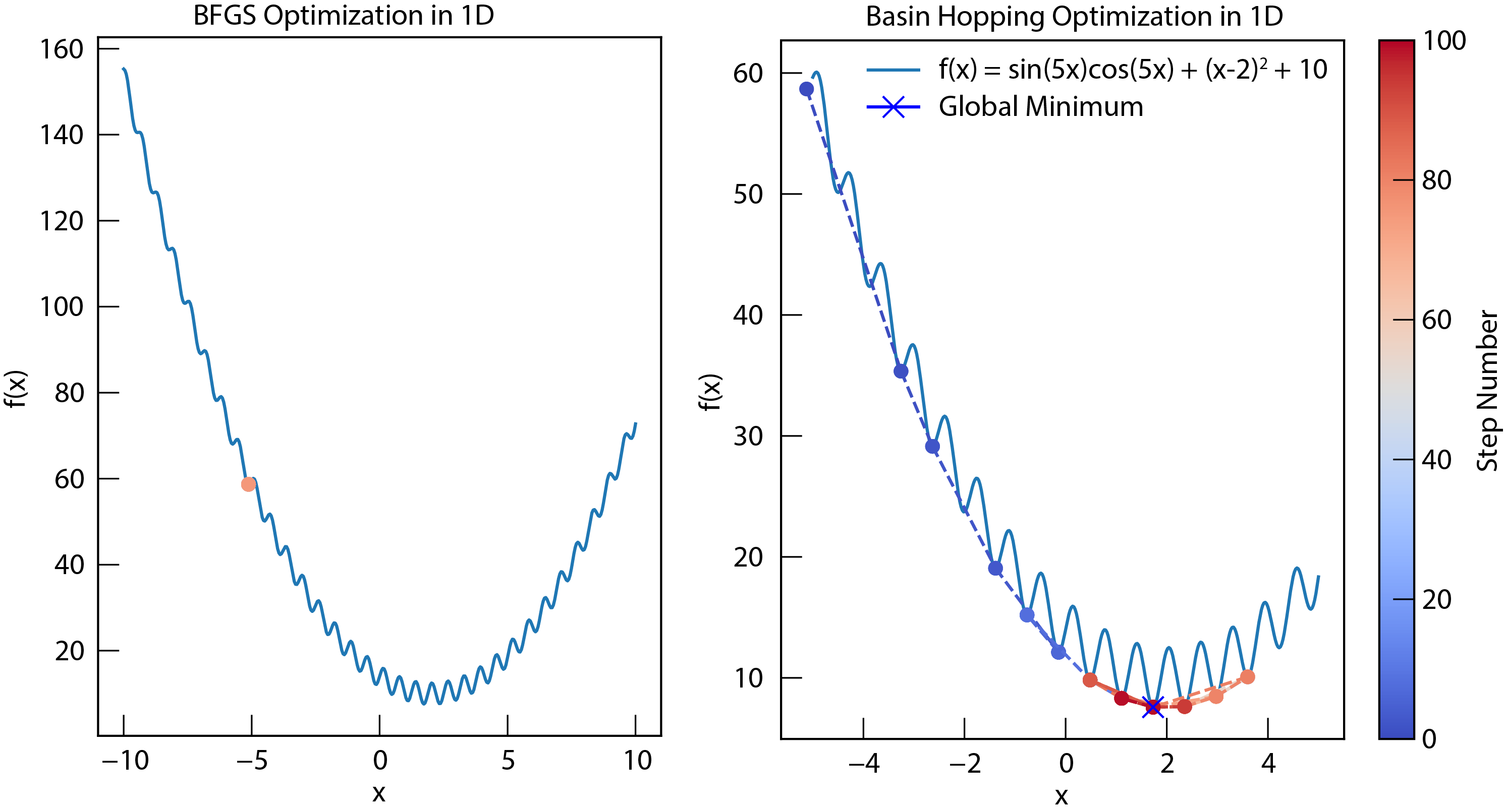
Basin hopping and comparison to BFGS. Basin hopping combines local optimization with random perturbations to escape local minima.
Basin hoopping combines local optimization with random perturbations. Transforms the objective function into a “staircase” of local minima.
It repeatedly performs local optimization (e.g., using BFGS) followed by a random perturbation of the variables (simulated to SA). Accepts or rejects moves based on a Metropolis criterion.
It is more efficient than SA for many problems, can handle rugged energy landscapes. However it still requires tuning parameters (e.g., the size of the perturbations).
Genetic Algorithm
These algorithms are inspired by biological evolution. They maintain a population of candidate solutions and use principles of selection, crossover, and mutation to evolve the population towards better solutions. GA’s explore the search space in a parallel and stochastic manner. The combination of selection, crossover, and mutation allows the algorithm to efficiently search for good solutions, even in complex, high-dimensional problems.
Algorithm
Initialization: Create an initial population of random solutions (often represented as “chromosomes” or bit strings).
Selection: Evaluate the “fitness” (objective function value) of each solution in the population. Select individuals for reproduction based on their fitness (e.g., using roulette wheel selection or tournament selection).
Crossover: Combine the “genetic material” of selected pairs of individuals to create new “offspring” solutions. This involves swapping parts of their representations.
Mutation: Introduce random changes to the offspring solutions. This helps to maintain diversity in the population and explore new regions of the search space.
Replacement: Replace some or all of the original population with the new offspring.
Repeat steps 2-5 for a specified number of generations or until a convergence criterion is met.
Other Global Optimization Methods
Particle Swarm Optimization (PSO): Inspired by the social behavior of birds flocking or fish schooling.
Bayesian Optimization: Uses a probabilistic model to guide the search, particularly useful for expensive objective functions.
Random Search: This is a simple baseline that samples candidate solutions randomly from the search space. It can be surprisingly effective in some high-dimensional problems, especially when function evaluations are cheap or easy to parallelize, but it does not rely on any general guarantee that large basins dominate the configurational space.