Introduction
In materials science and engineering, we’re constantly searching for better materials. Better might mean stronger, lighter, more conductive, more stable, cheaper to produce, or a combination of these properties. “Better” almost always translates to finding the optimal value of some property or combination of properties. This is where optimization comes in.
Optimization, in a mathematical sense, is the process of finding the input values to a function that result in either the minimum or maximum output value of that function. We call this function we’re trying to minimize or maximize the objective function (sometimes also called the cost function or energy function).
Think about it:
Designing a new alloy: We want to find the optimal composition (percentages of different elements) that maximizes strength and minimizes weight.
Predicting crystal structures: We want to find the atomic arrangement with the lowest potential energy, as this represents the most stable structure.
Optimizing a synthesis process: We might want to find the reaction conditions (temperature, pressure, concentration) that yield the highest product purity in the shortest time.
Training Machine Learning Models: We optimize parameters of model to minimize loss, which makes model’s prediction close to real data.
In all these cases, we have a defined objective function (strength, energy, purity, loss, etc.) and a set of variables we can control (composition, atomic positions, reaction conditions, model’s parameters). Optimization is the systematic process of exploring the space of these variables to find the “best” possible outcome according to our objective function.
Basic Concepts and Overview
Before diving into specific algorithms, let’s define some key concepts:
Objective Function
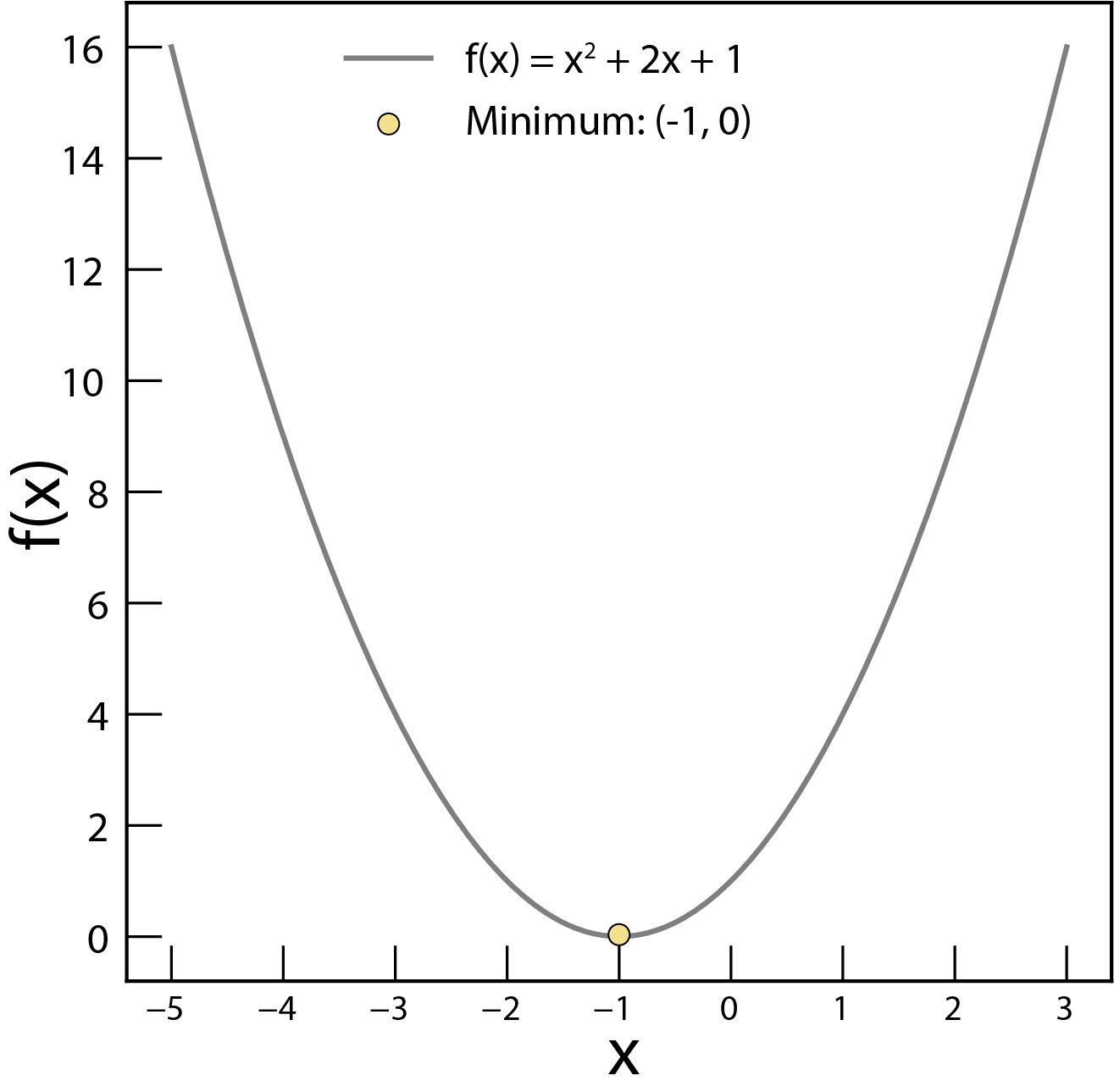
Object function . The minimum value of this function is 0 at .
This is the function we want to minimize or maximize. x represents the input variables (often a vector). For example:
f(x)could be the total energy of a crystal structure, wherexrepresents the positions of all the atoms.f(x)could be the cost of manufacturing a material, wherexrepresents the processing parameters.f(x)could be the loss function, wherexrepresents the parameters.
Variables
These are the parameters we can adjust to influence the objective function. They can be:
Continuous: Like temperature or pressure, which can take on any value within a range.
Discrete: Like the choice of a specific element in an alloy (e.g., choosing between aluminum, iron, or copper).
Categorical: Representing distinct categories, like crystal structure type (FCC, BCC, HCP).
Constraints
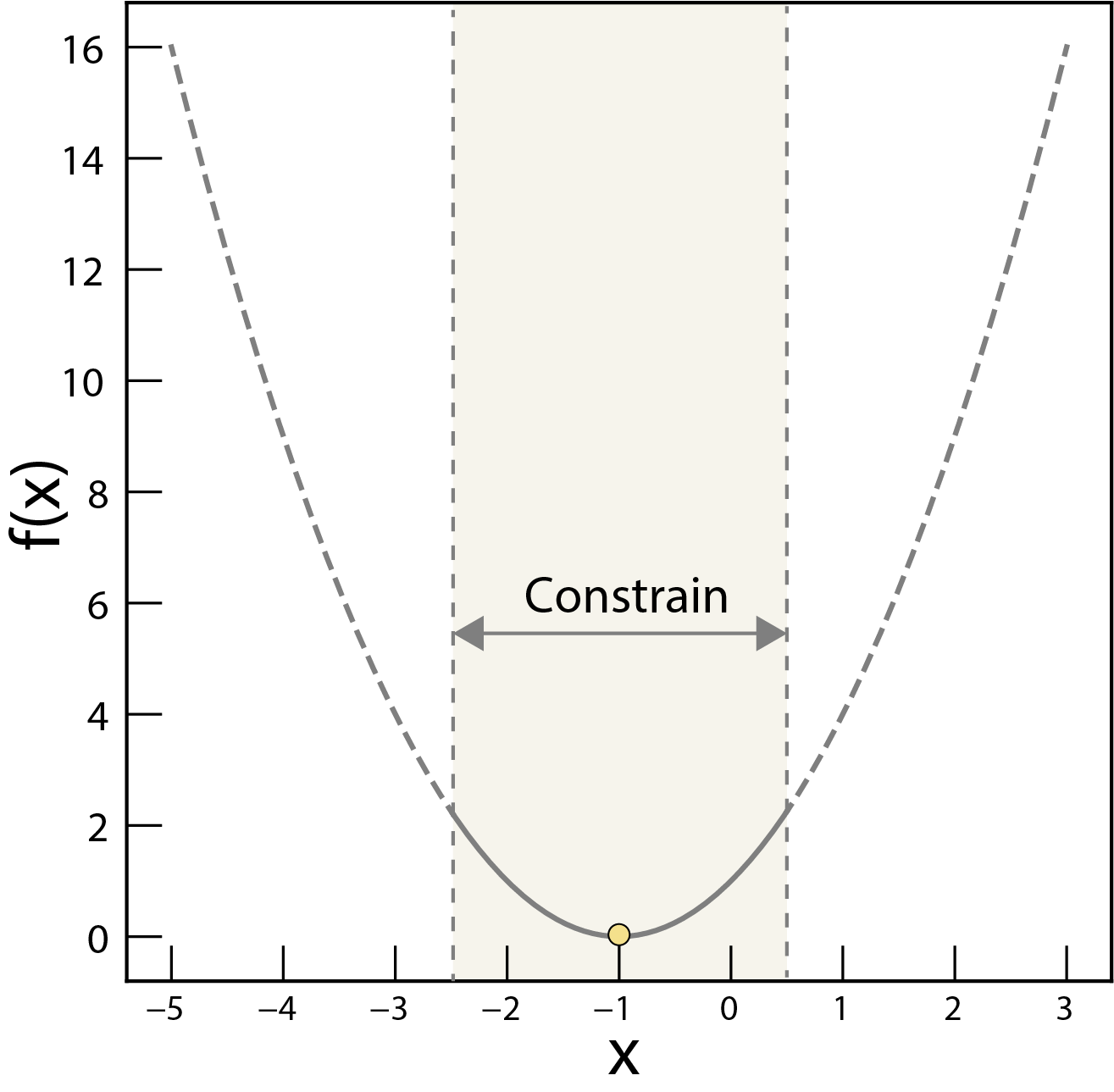
The constrains of the optimization problem. Here, the feasible region is constrained by the inequality and .
Often, we can’t simply choose any value for our variables. Constraints define the allowed range or relationships between variables. Examples:
Composition constraints: The percentages of all elements in an alloy must sum to 100%.
Temperature limits: A reaction might only be feasible within a certain temperature range.
Non-negativity: Concentrations of chemical species cannot be negative.
Local vs. Global Optima
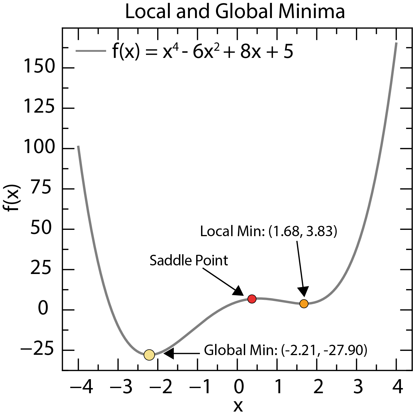
Local and global minima of a function. The global minimum is the lowest point in the entire search space, while local minima are lower than nearby points.
Local Minimum: A point where the objective function is lower than all nearby points. Imagine a small dip in a hilly landscape.
Global Minimum: The absolute lowest point of the objective function across the entire search space. This is the deepest valley in our landscape.
Finding the global minimum is generally much harder than finding a local minimum. Many optimization algorithms can get “stuck” in local minima, failing to find the true global optimum.
Convexity
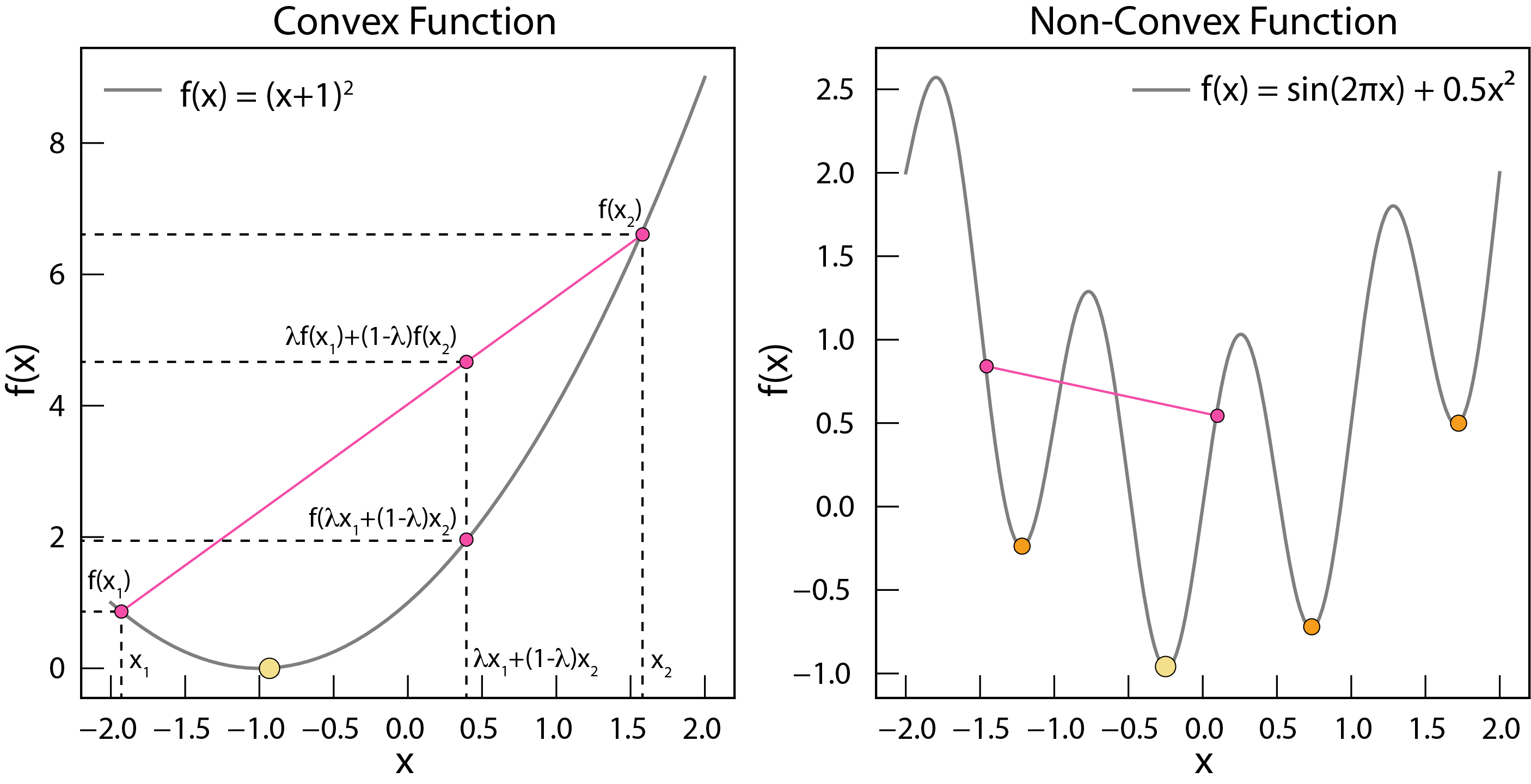
Convex and non-convex functions. Convex functions have only one minimum, which is the global minimum. Non-convex functions have multiple local minima.
A function is convex if, for any two points within its domain, the line segment connecting those points lies entirely above or on the function’s curve. Mathematically:
for any , in the domain and any between 0 and 1.
Convex functions are “nice” because they have only one minimum, which is the global minimum. If a function is non-convex (has multiple bumps and valleys), finding the global minimum is much more challenging.
Gradient
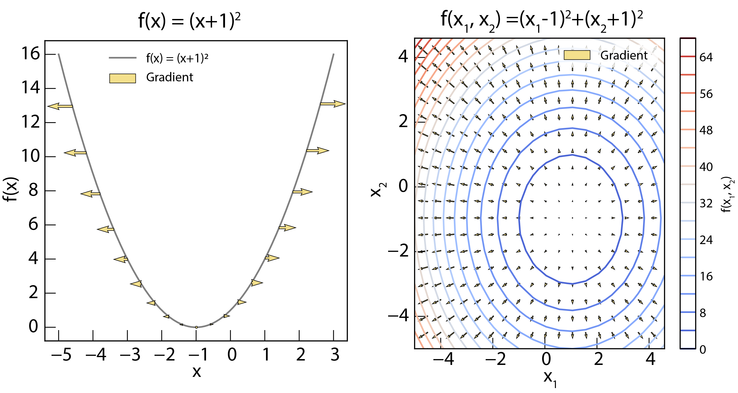
Left panel: The gradient of 1D function . The gradient is shown as arrows, pointing in the opposite direction of steepest ascent. Right panel: The gradient of 2D function . The gradient is shown as vectors, pointing in the direction of steepest ascent.
The gradient, denoted by , is a vector that points in the direction of the steepest ascent of the function at a given point. Its components are the partial derivatives of the function with respect to each variable:
The negative gradient, , points in the direction of steepest descent. This is fundamental to many optimization algorithms. The gradient can be computed using numerical differentiation or symbolic differentiation.
Hessian
The Hessian matrix is the square matrix of second-order partial derivatives of a scalar-valued function.
The Hessian provides information about the local curvature of the function. At a stationary point where , a positive definite Hessian indicates a local minimum, a negative definite Hessian indicates a local maximum, and a Hessian with both positive and negative eigenvalues indicates a saddle point. The Hessian can be computed using numerical differentiation or symbolic differentiation, but it can be computationally expensive for high-dimensional functions.
Challenges
Optimizing materials presents significant challenges due to the inherent complexity of materials and the computational demands involved.
High Dimensionality
Material properties are influenced by numerous factors (composition, structure, processing), creating a vast, high-dimensional search space. This “curse of dimensionality” makes finding the global optimum exponentially harder.
Non-Convexity
The relationship between a material’s properties and its defining variables (the objective function) is often non-convex, exhibiting multiple local minima. Algorithms can get trapped in these local minima, mistaking them for the global optimum.
Computational Cost
Evaluating the objective function frequently requires computationally expensive simulations (e.g., DFT, MD) or experiments. This limits the number of evaluations, hindering thorough exploration of the search space.
Discrete and Continuous Variables
Optimization problems often involve both discrete variables (e.g., element choices, crystal structure type) and continuous variables (e.g., composition, temperature). This mixture requires specialized algorithms.
Noisy Objective Functions
Experimental measurements and computational simulations are subject to noise. This makes it harder to determine the true objective function value and can mislead optimization algorithms.
Physical and Chemical Constraints
Optimization must adhere to physical and chemical constraints (charge neutrality, phase stability, stoichiometry, manufacturability), limiting the search space.
Multi-Objective Optimization
Optimizing multiple properties simultaneously (e.g., strength and ductility) leads to a set of Pareto-optimal solutions (the Pareto front), where improving one objective worsens another. This adds complexity to decision-making. One common way to convert a multi-objective problem into a single-objective one is to use a weighted sum, for example
but this is only one scalarization strategy and may not recover all Pareto-optimal solutions when the Pareto front is non-convex.