Transition State Theory
In materials science, we’re often interested not just in stable states (minima on the potential energy surface) but also in the transition states that connect them. Transition states are saddle points on the potential energy surface, representing the energy barrier that must be overcome for a system to move from one stable state to another. Examples include:
Chemical Reactions: The transition state represents the highest-energy point along the reaction pathway, corresponding to the activated complex.
Diffusion: An atom moving from one lattice site to another must pass through a transition state.
Phase Transformations: The transition state represents the configuration with the highest energy during the transformation from one phase to another (e.g., from FCC to BCC).
Knowing the energy of the transition state (the activation energy) is crucial for understanding the kinetics of these processes. The minimum energy path (MEP) is the path connecting two minima that passes through the transition state with the lowest possible energy barrier. The Nudged Elastic Band (NEB) method is a powerful technique for finding the MEP.
Nudged Elastic Band Method
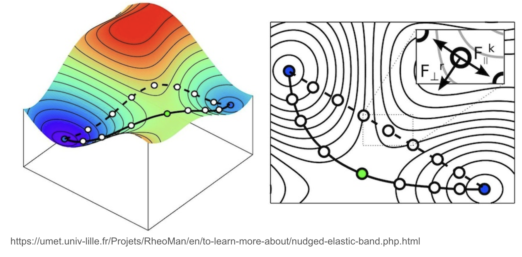
The potential energy surface showing stable states, transition states, and the minimum energy path (MEP). In NEB, a series of images are used to represent the path between the initial and final states. The forces perpendicular to the band are projected to find the MEP.
NEB creates a series of intermediate configurations (“images”) between the initial and final states, forming a “band” or “chain” of states. These images are connected by fictitious “springs,” and the forces acting on the images are carefully modified to guide the band towards the MEP.
Algorithm
Initialization: Create a set of N images (including the initial and final states) along an initial guess for the path. A simple linear interpolation between the initial and final states is often used as the starting point. Denote the positions of the images as , where is the initial state and is the final state.
Spring Forces: Introduce spring forces between adjacent images. These forces tend to keep the images evenly spaced along the band. The spring force on image i is given by:
where is the spring constant (a parameter that controls the strength of the spring forces), is the distance between image *i-and image i+1, and is the unit tangent vector to the band at image i.
A common approximation for the tangent is: . More sophisticated tangent estimates are also used (see below).
Force Projection: This is the crucial step that distinguishes NEB from a simple elastic band method. The true forces acting on each image (the negative gradient of the potential energy, ) are projected to prevent the band from simply sliding down to the initial or final minima.
Calculate true force: .
Project out the parallel component of the true force: The component of the true force parallel to the band is removed. This prevents the images from sliding down along the band towards the minima. The force perpendicular to the band is:
Project out the perpendicular component of the spring force: The component of the spring force perpendicular to the band is removed. This allows the band to find the MEP without being constrained to a straight line.
Total Force: The total force acting on image i is the sum of the projected true force and the projected spring force:
Optimization: The positions of the images (excluding the fixed initial and final states) are updated by moving them in the direction of the total force. This can be done using any standard optimization algorithm, such as:
Gradient Descent:
Velocity Verlet: A common choice in molecular dynamics simulations.
BFGS or other quasi-Newton methods: Can be more efficient than gradient descent.
Iteration: Repeat steps 3-5 until the forces on the images are sufficiently small (i.e., the system has converged to the MEP).
Tangent Estimation: The choice of the tangent vector, , can affect the convergence of the NEB method. Several improved tangent estimates exist:
Energy-weighted tangent:
Bicparabolic interpolation.
Climbing Image NEB (CI-NEB):
The standard NEB method tends to distribute images evenly along the MEP, which can result in poor resolution around the transition state. The Climbing Image NEB (CI-NEB) modification addresses this issue.
In CI-NEB, the image with the highest potential energy is identified (the “climbing image”). The spring forces acting on this image are removed, and the component of the true force parallel to the band is inverted. This drives the climbing image up the potential energy surface towards the saddle point.
Modified Force: For the climbing image, c, the force is: Notice that there is no spring force, and the parallel component of the true force is added instead of subtracted. This pushes the image uphill along the band.
Advantages: CI-NEB provides a much more accurate determination of the transition state energy and configuration.
Algorithm: The algorithm is the same as standard NEB, except for the modified force calculation for the climbing image. The climbing image is identified at each iteration.