Interface
Interfaces represent the boundaries between different materials or phases of the same material. These boundaries can manifest as surfaces, grain boundaries, or interfaces between distinct chemical compositions. The nature of the atomic arrangement at an interface significantly influences the material’s overall behavior.
Interfaces can be broadly categorized based on the degree of lattice matching between the adjacent materials: coherent, incoherent, and semi-coherent. A coherent interface exhibits perfect lattice matching, while an incoherent interface displays a complete mismatch. Semi-coherent interfaces represent an intermediate state, accommodating some degree of mismatch through periodic defects.
Interfaces play a crucial role in determining material properties and performance, as illustrated by the following examples:
- Hall-Petch Effect: The presence of grain boundaries in polycrystalline materials impedes dislocation motion, leading to increased strength and hardness with decreasing grain size. This phenomenon is known as the Hall-Petch effect.
- Energy Storage: In rechargeable batteries, the solid-solid or solid-liquid interfaces are critical for ion transport and electrochemical reactions, directly impacting battery performance.
- Electronics: Heterojunctions, such as GaN/InGaN, create interfaces with tailored electronic properties, enabling enhanced light emission efficiency in optoelectronic devices.
The interface region represents a transition zone where the properties of the adjacent materials change. This region may exhibit distinct mechanical, electrical, or thermal characteristics compared to the bulk materials.
Surface/Slab
A slab model is a computational technique used to simulate surfaces and interfaces, enabling the study of phenomena like adsorption and catalysis. When constructing a slab model, several key parameters must be carefully considered:
- Bulk Structure: The starting point is an accurate representation of the bulk material’s crystal structure.
- Miller Index: This specifies the orientation of the surface being modeled. Different Miller indices correspond to different surface terminations, each with its own unique atomic arrangement and properties.
- Slab Thickness: The slab must be thick enough to represent the bulk-like behavior of the material, while also being computationally tractable.
- Vacuum Thickness: A sufficient vacuum layer is needed to minimize interactions between periodic images of the slab.
- Bonds to Cut/Keep: Deciding which bonds to cleave when creating the surface can influence the surface energy and stability.
The surface of a material represents the boundary where it interacts with its surroundings. Surface properties often differ significantly from those of the bulk material due to the altered atomic coordination and electronic structure. These differences play a crucial role in phenomena like catalysis, corrosion, and thin film growth.
Surface Energy
Surface energy is a measure of the excess energy associated with creating a surface. It arises from the broken bonds and unsaturated coordination of atoms at the surface. A higher surface energy indicates a less stable surface. Surface energy can be computed using the following formula:
where:
- γ is the surface energy.
- is the surface area of the surface.
- is the total energy of the slab.
- is the energy of the equivalent number of atoms in the bulk. The factor of 1/2 accounts for the fact that the slab has two surfaces.
Tasker Classification of Slabs
Tasker classification provides a way to categorize slabs based on their electrostatic properties:
- Type I: These slabs are charge neutral and possess no dipole moment perpendicular to the surface. They are typically the most stable.
- Type II: These slabs are also charge neutral, but they exhibit a dipole moment. While generally stable, they may exhibit surface reconstructions to minimize the dipole.
- Type III: These slabs are non-charge neutral and possess a dipole moment. They are inherently unstable and require surface modifications or charge compensation to achieve stability.
Understanding Tasker’s classification helps in predicting the stability and behavior of different surface terminations.
Particle Morphology
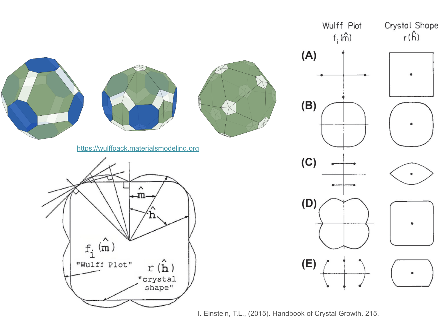
Wulff shape example and construction.
The shape of a small particle, like a nanocrystal, isn’t always a perfect sphere. Instead, it often adopts a specific morphology dictated by the energetics of its surfaces. At equilibrium, this morphology can be predicted using the Wulff construction.
Imagine plotting the surface energy (γ) of a crystal as a function of its orientation. This plot, often visualized in polar coordinates, is known as the Wulff plot. Each point on this plot represents a specific crystallographic plane (defined by its Miller indices, hkl) and its corresponding surface energy.
The Wulff construction then proceeds as follows: for every point P on the Wulff plot, visualize a plane that is perpendicular to the vector connecting P to the origin (center) of the plot. The internal envelope formed by the intersection of all these planes defines the equilibrium crystal shape. In simpler terms, the Wulff construction identifies the shape that minimizes the total surface energy of the particle.