ML Tasks and Algorithms
Machine learning models learn from data by optimizing objective functions using mathematical techniques such as gradient descent, entropy minimization, or probabilistic inference. Below, we provide a deeper dive into the core mathematical formulations and training methods for major ML algorithms.
Supervised Learning
Supervised learning algorithms use labeled data , where is the input feature vector and is the corresponding label. The goal is to learn a mapping function that minimizes the loss function over the training set.
Linear Regression
Linear regression is a simple supervised learning algorithm used for regression tasks. It assumes a linear relationship between the input features and the target variable. The model can be expressed as:
where is the weight vector, is the input feature vector, and is the bias term. We can use the mean squared error (MSE) as the loss function.
The optimal weights and bias can be found using gradient descent or its variants: Stochastic gradient descent (SGD), mini-batch gradient descent, etc. The update rule for the weights and bias can be done using gradient descent.
Logistic Regression
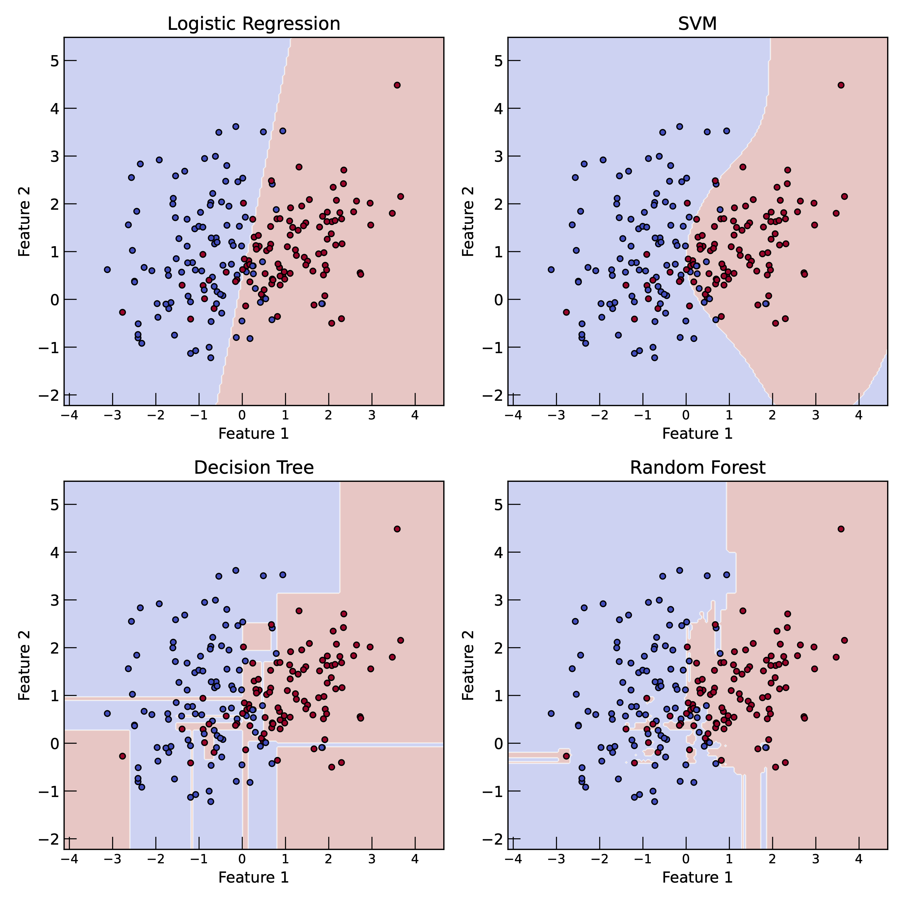
Classification examples of different algorithms: logistic regression, SVM, decision trees, and random forests. The decision boundaries are shown in the plots. The data points are colored according to their class labels. The decision boundaries are determined by the model’s parameters and the training data. The models aim to find the optimal decision boundary that separates different classes in the feature space.
Logistic regression is a supervised learning algorithm used for binary classification tasks. It models the probability of the positive class using the logistic function:
where is the probability of the positive class given the input feature vector . The loss function for logistic regression is the binary cross-entropy loss. The optimal weights and bias can be found using gradient descent or its variants. The update rule for the weights and bias can be done using gradient descent.
Support Vector Machines (SVM)
Support Vector Machines (SVM) are supervised learning algorithms used for classification and regression tasks. They aim to find the optimal hyperplane that separates different classes in the feature space. The SVM optimization problem can be formulated as:
where is the regularization parameter, are slack variables that allow for misclassification, and is the number of samples in the training set. The constraints ensure that the samples are correctly classified:
The optimal hyperplane is determined by the support vectors, which are the data points closest to the decision boundary. The SVM can also be extended to non-linear classification using kernel functions, which map the input data into a higher-dimensional space.
The loss function for SVM can be expressed as the hinge loss. The hinge loss penalizes misclassified samples and encourages a margin between the classes.
Decision Trees & Random Forests
Decision trees are supervised learning algorithms used for classification and regression tasks. They recursively partition the feature space based on the input features to create a tree-like structure. Each internal node represents a feature, each branch represents a decision rule, and each leaf node represents a class label or a continuous value.
The loss function for decision trees can be based on the Gini impurity or entropy for classification tasks, and mean squared error (MSE) for regression tasks. The objective is to minimize the loss function (Gini impurity) by selecting the best feature and threshold at each node.
Random forests are an ensemble learning method that combines multiple decision trees to improve the model’s performance and reduce overfitting. The random forest algorithm constructs multiple decision trees using bootstrapped samples of the training data and averages their predictions for regression tasks or uses majority voting for classification tasks.
Neural Networks
Neural networks are a class of supervised learning algorithms inspired by the structure and function of the human brain. They consist of interconnected nodes (neurons) organized into layers: input layer, hidden layers, and output layer. Each neuron applies a non-linear activation function to the weighted sum of its inputs. A simple neural network is also called a multi-layer perceptron (MLP) or vanilla neural network.
The output of a neuron can be expressed as:
where is the activation function, is the weight vector, is the input feature vector, and is the bias term. Common activation functions include sigmoid, ReLU (Rectified Linear Unit), and tanh.
How to Choose Activation Functions (click)
Choosing the right activation function for a neural network depends on the task and the architecture of the network. Here are some common guidelines:
Sigmoid: Use for binary classification tasks or the output layer of a network where probabilities are required. However, it can suffer from vanishing gradients in deep networks.
ReLU (Rectified Linear Unit): A popular choice for hidden layers due to its simplicity and efficiency. It helps mitigate the vanishing gradient problem but can suffer from “dead neurons” if gradients become zero.
Leaky ReLU: A variant of ReLU that addresses the “dead neuron” issue by allowing a small gradient for negative inputs.
Tanh: Use for hidden layers when the data is centered around zero. It can also suffer from vanishing gradients in deep networks.
Softmax: Use in the output layer for multi-class classification tasks to produce probabilities for each class.
The choice of activation function can significantly impact the training process and the performance of the model. Experimentation and validation are often necessary to determine the best activation function for a specific problem.
The loss function for neural networks can be similar to that of linear regression or logistic regression, depending on the task (regression or classification). The optimization process involves minimizing the loss function using gradient descent or its variants.
The objective function for a neural network can be expressed as:
where is the objective function, is the loss function, and is the regularization term. The regularization term helps prevent overfitting by penalizing complex models.
The backpropagation algorithm is used to compute the gradients of the loss function with respect to the weights and biases in the network. The weights and biases can be updated using the gradient descent.
Neural network is highly flexible and we can choose different form of the objective function depending on the task. For example, for classification tasks, we can use cross-entropy loss, while for regression tasks, we can use mean squared error (MSE) loss.
Deep Learning
Deep learning is a subfield of machine learning that focuses on neural networks with many layers (deep networks). Deep learning models can learn hierarchical representations of data, allowing them to capture complex patterns and relationships. They are particularly effective for tasks such as image recognition, natural language processing, and speech recognition.
Unsupervised Learning
Unsupervised learning algorithms learn from unlabeled data, where the goal is to discover patterns or structures in the data. Common unsupervised learning tasks include clustering, dimensionality reduction, and anomaly detection.
K-Means Clustering
K-Means clustering is an unsupervised learning algorithm used for clustering tasks. It aims to partition the data into clusters by minimizing the within-cluster variance. The algorithm iteratively updates the cluster centroids and assigns data points to the nearest centroid until convergence.
The objective function for K-Means clustering can be expressed as:
where is the objective function, is the number of clusters, is the set of data points in cluster , and is the centroid of cluster . The algorithm alternates between assigning data points to clusters and updating the centroids until convergence.
Principal Component Analysis (PCA)
Example of K-Means clustering. Points are colored according to their assigned clusters. The centroids of the clusters are marked with crosses. The algorithm iteratively updates the centroids and assigns points to the nearest centroid until convergence.
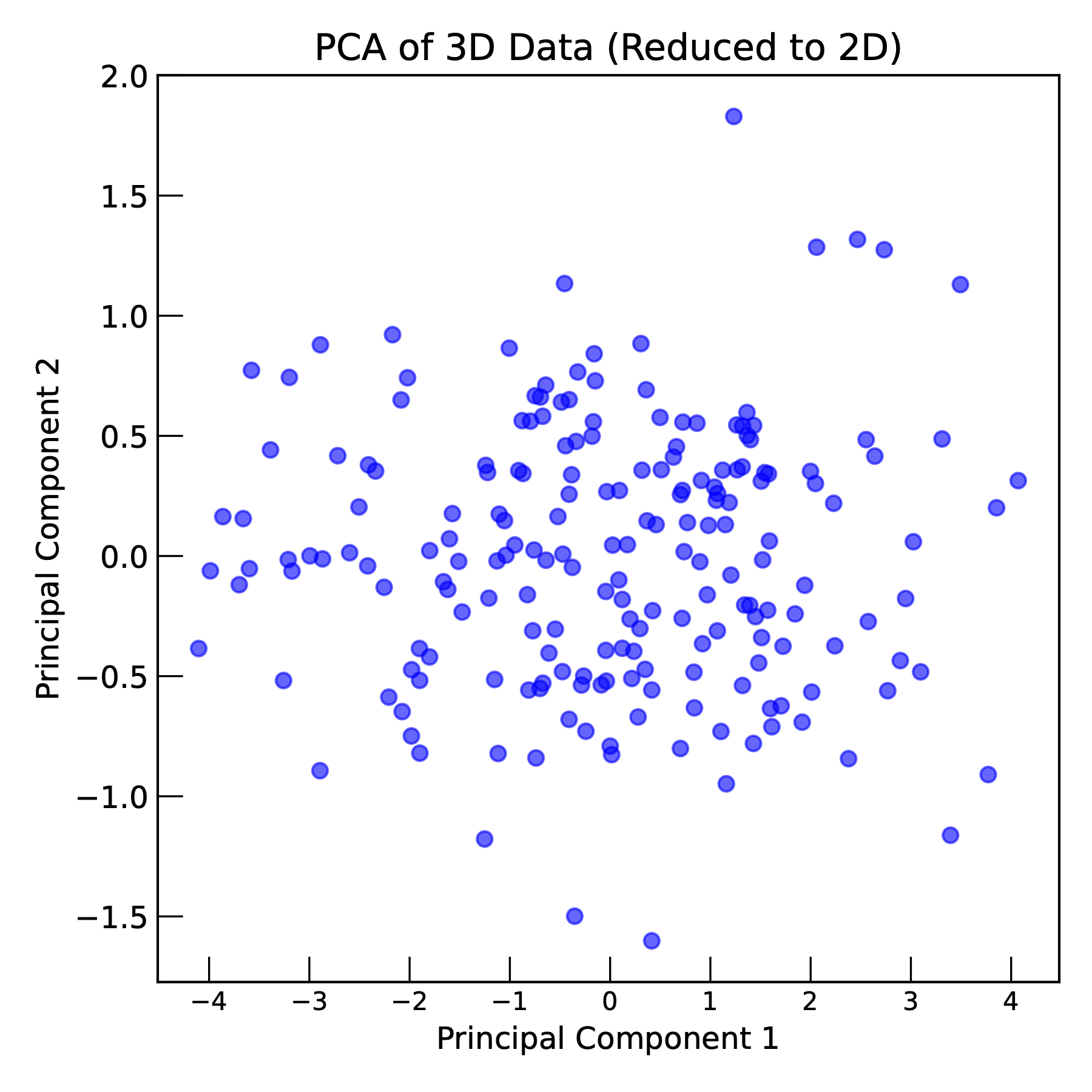
Principal Component Analysis (PCA) is an unsupervised learning algorithm used for dimensionality reduction. It aims to find the directions (principal components) that maximize the variance in the data. PCA can be expressed as an optimization problem:
where is the direction of the principal component, is the input feature vector, and is the number of samples in the dataset. The optimal direction can be found by solving the eigenvalue problem for the covariance matrix of the data.
The covariance matrix can be expressed as:
where is the covariance matrix, is the input feature vector, and is the mean of the data. The eigenvalues and eigenvectors of the covariance matrix represent the variance and direction of the principal components, respectively.
PCA transforms the original data into a new coordinate system where the axes correspond to the principal components. The first principal component captures the maximum variance, the second captures the second maximum variance orthogonal to the first, and so on. By selecting a subset of the principal components, PCA can reduce the dimensionality of the data while preserving most of its variance.