Model
A machine learning model is a mathematical representation of the relationship between input features and output labels. The model can be expressed as a function , where is the input feature vector. The model parameters (weights and biases) are learned from the training data to minimize the loss function.
Parameters and Hyperparameters
Parameters are the internal variables of the model that are learned during the training process. They include weights and biases in neural networks, coefficients in linear regression, and support vectors in SVMs. The parameters are adjusted to minimize the loss function during training. For example, in linear regression (), the parameters are the weights () and bias () that define the linear relationship between the input features and the target variable.
Hyperparameters are parameters that are set before the training process begins. They control the learning process and can significantly impact the model’s performance. Examples of hyperparameters include the learning rate, batch size, number of epochs, and regularization strength. Hyperparameters are typically tuned using techniques such as grid search or random search.
Loss Function
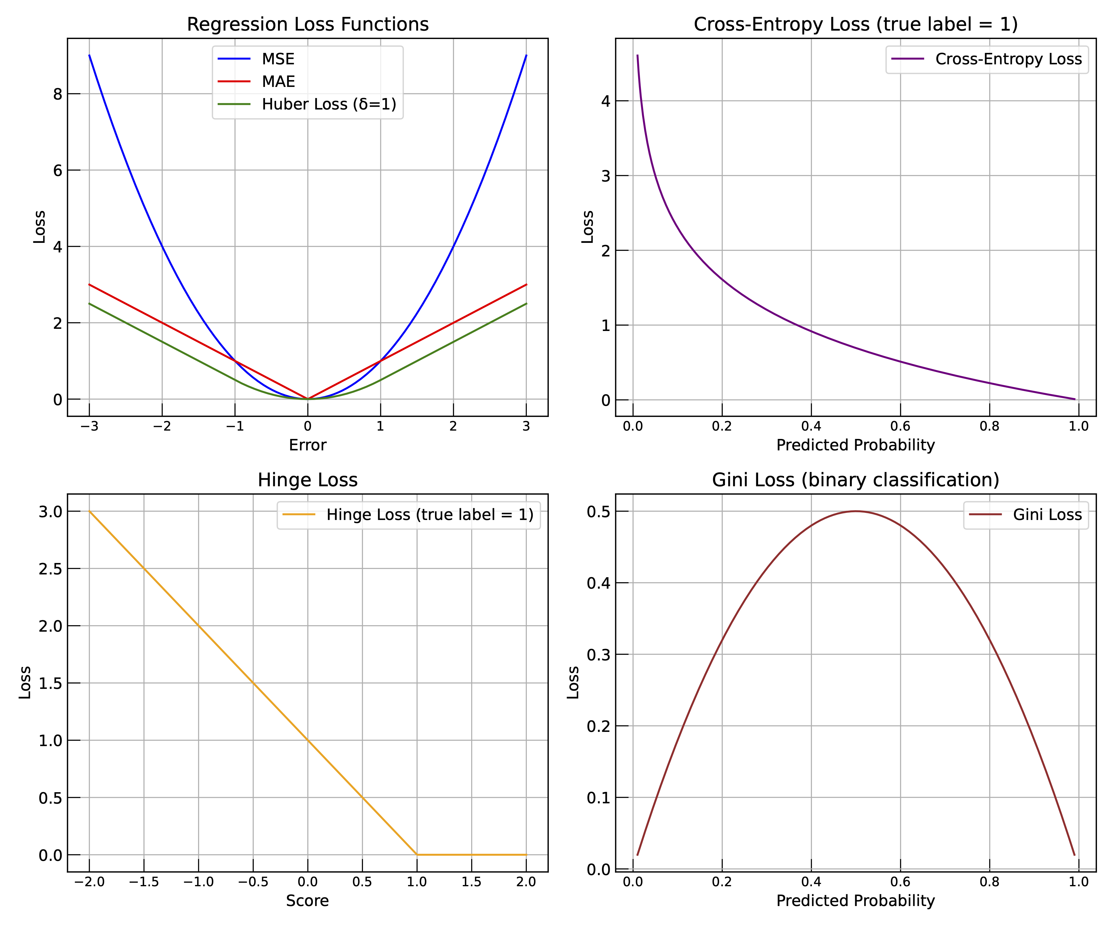
Commonly used loss functions. The loss function quantifies the difference between the predicted output and the true output, while the objective function includes the loss function and any regularization terms. Loss function can be varied depending on the type of problem being solved (e.g., regression, classification).
The loss function, also known as the cost function or objective function, quantifies how well a machine learning model performs on a given dataset. It measures the difference between the predicted output and the true output. The goal of training a machine learning model is to minimize this loss function.
Mean Squared Error (MSE)
The Mean Squared Error (MSE) is a commonly used loss function for regression tasks. It calculates the average of the squared differences between the predicted values and the actual values. The MSE can be expressed mathematically as:
where is the true output, is the predicted output, and is the number of samples in the dataset. The MSE penalizes larger errors more than smaller ones, making it sensitive to outliers.
Mean Absolute Error (MAE)
The Mean Absolute Error (MAE) is another loss function used for regression tasks. It calculates the average of the absolute differences between the predicted values and the actual values. The MAE can be expressed mathematically as:
where is the true output, is the predicted output, and is the number of samples in the dataset. The MAE is less sensitive to outliers compared to the MSE, making it a robust choice for certain applications.
Huber Loss
Huber loss is a combination of MSE and MAE. It is less sensitive to outliers than MSE and is defined as:
where is the true output, is the predicted output, and is a threshold parameter. The Huber loss behaves like MSE when the error is small and like MAE when the error is large, making it a good choice for regression tasks with outliers.
Cross-Entropy Loss
Cross-entropy loss is commonly used for classification tasks. It measures the dissimilarity between the predicted probability distribution and the true distribution. For binary classification, the cross-entropy loss can be expressed as:
where is the true label (0 or 1), is the predicted probability of the positive class, and is the number of samples in the dataset. The cross-entropy loss penalizes incorrect predictions more heavily than correct ones, making it suitable for classification tasks.
Hinge Loss
Hinge loss is commonly used for “maximum-margin” classification, most notably with support vector machines (SVMs). It is defined as:
where is the true label (1 or -1), is the predicted output, and is the number of samples in the dataset. The hinge loss encourages the model to make predictions that are not only correct but also have a margin of confidence.
Gini Impurity
Gini impurity is a measure of how often a randomly chosen element from the set would be incorrectly labeled if it was randomly labeled according to the distribution of labels in the subset. It is used in decision trees to determine the best split at each node. The Gini impurity can be expressed as:
where is the number of classes and is the proportion of instances belonging to class in the subset. The Gini impurity ranges from 0 (pure) to 0.5 (impure).
Regularization
The optimization process involves finding the optimal parameters of the model that minimize the loss function. The optimization algorithm iteratively updates the model parameters based on the gradients of the loss function with respect to the parameters.
The objective function is a broader term that encompasses the loss function and any additional regularization terms. The objective function can be expressed as:
where is the objective function, is the regularization term, and and are the model parameters (weights and biases). The regularization term helps prevent overfitting by penalizing complex models.
The regularization term can take various forms, such as L1 (Lasso) or L2 (Ridge) regularization. The choice of regularization term depends on the specific problem and the desired properties of the model.
Optimization
The optimization process involves finding the optimal parameters and that minimize the objective function. This is typically done using gradient descent or its variants, such as stochastic gradient descent (SGD) or mini-batch gradient descent.
The optimization process can be expressed mathematically as:
where is the learning rate, is the weight vector, and is the gradient of the objective function with respect to the weights. The learning rate controls the step size in the optimization process.
The optimization process iteratively updates the model parameters until convergence, i.e., when the change in the objective function is below a certain threshold or when a maximum number of iterations is reached.
Concept
There are some terminologies that are frequently used in training process:
Epoch: One complete pass through the entire training dataset. Usually, multiple epochs are required to train a model effectively.
Batch: A subset of the training dataset used to update the model parameters during each iteration. This is important for GPU acceleration, as it allows for parallel processing of multiple samples.
Iteration: One update of the model parameters based on a batch of data.
Learning Rate: A hyperparameter that controls the step size in the optimization process. A small learning rate may lead to slow convergence, while a large learning rate may cause overshooting and divergence.
Convergence: The process of reaching a stable state where the model parameters no longer change significantly.
Choose the Right Model
Choosing the right model for a specific task is crucial for achieving good performance. The choice of model depends on various factors, including the nature of the data, the complexity of the problem, and the desired interpretability of the model.
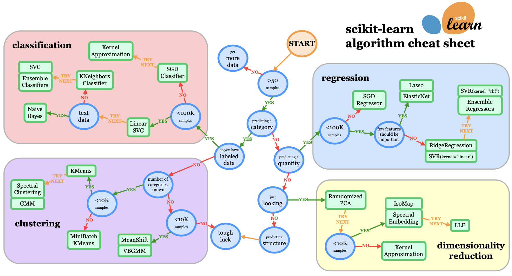
The flowchart illustrates the process of choosing the right model for a specific task. It starts with understanding the data and the problem, followed by selecting the appropriate model type.