Thermodynamics
Once the properties of a large number of structures have been calculated, the next step is to analyze the data to identify stable and potentially synthesizable materials. Thermodynamics provides the framework for this analysis.
Formation Energy
The formation energy of a compound is a key quantity for assessing the stability of a compound at 0 K. It is defined as the energy difference between the compound and its constituent elements in their standard reference states.
where is the total energy of the compound per formula unit, calculated using DFT or a force field. and are the total energies per atom of the elements A and B in their standard reference states. The reference state is typically the most stable form of the element at standard conditions (e.g., for Li, it is body-centered cubic Li metal; for O, it is the O molecule). The formation energy is typically expressed per formula unit (f.u.) of the compound.
A negative formation energy indicates that the compound is stable with respect to its constituent elements. The more negative the formation energy, the more stable the compound is. A positive formation energy suggests that the compound is unstable and will decompose into its constituent elements.
Convex Hull
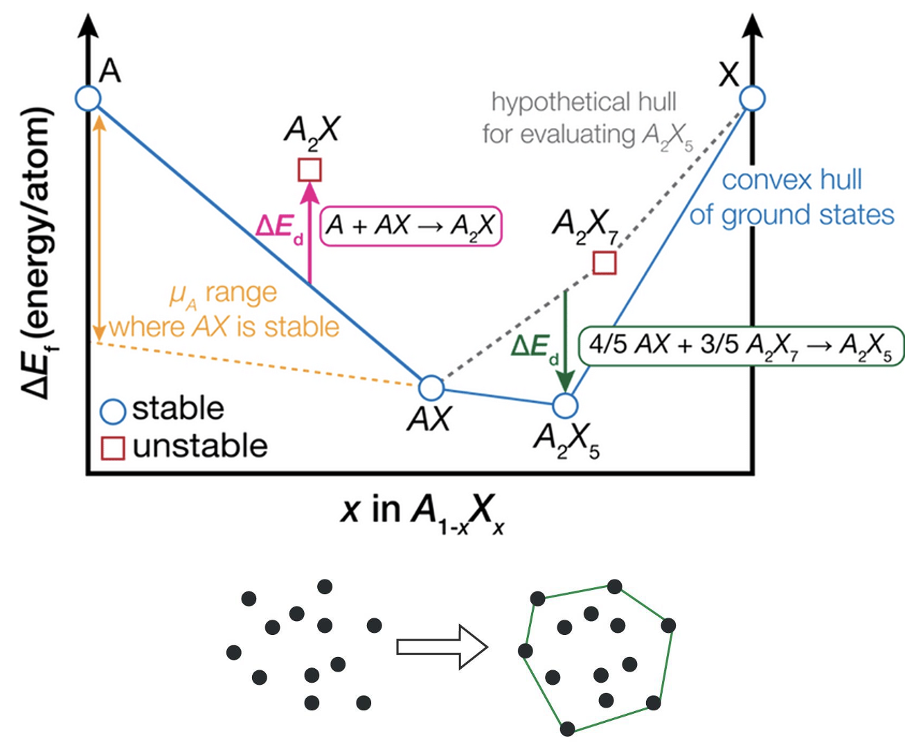
Convex hull construction for a binary system. The points represent the formation energies of different compounds. The compounds that lie on the convex hull are stable phases, while those above the hull are unstable. Reproduced from Bartel.
For systems with more than two components (e.g., ternary or quaternary systems), the concept of the convex hull is used to determine phase stability. The convex hull is a geometric construct that represents the lowest-energy phases at different compositions.
Construction of the convex hull involves the following steps:
Plot Formation Energies: Plot the formation energies of all calculated compounds as a function of composition. For a binary system (A-B), this is a simple 2D plot with the composition (e.g., the atomic fraction of B) on the x-axis and the formation energy on the y-axis. For a ternary system (A-B-C), this is a 3D plot (a ternary diagram).
Identify the Lowest-Energy Surface: The convex hull is the “lowest-energy surface” that connects the points representing the most stable compounds. It is formed by connecting the points in such a way that all other points lie above the surface.
Compounds that lie on the convex hull represent stable phases at 0 K. These compounds are in thermodynamic equilibrium whereas compounds that lie above the convex hull are unstable or metastable. They will tend to decompose into a mixture of phases that lie on the hull. The vertical distance of a point above the hull () represents the driving force for decomposition.
Practically, the convex hull can be constructed using packages like SciPy or pymatgen, which provide functions for calculating the convex hull from a set of formation energies.
For example, consider a binary system A-B. Suppose we have calculated the formation energies of several compounds: A, A3B, A2B, AB, AB2, AB3, and B. After plotting these energies and constructing the convex hull, we might find that A, A2B, AB2, and B lie on the hull, while A3B and AB lie above it. This means that A, A2B, AB2, and B are stable phases, while A3B and AB are unstable and will decompose into mixtures of the stable phases.
Thermodynamic Potentials
The convex hull analysis described above is strictly valid only at 0 K. At finite temperatures, entropic contributions become important and can stabilize compounds that are unstable at 0 K. The Gibbs free energy is the appropriate thermodynamic potential to consider at finite temperatures, defined as:
where is the total energy, is the enthalpy, is the entropy, is the temperature, and is the pressure-volume term.
For solid-state materials at ambient pressure, the pV term is usually negligible, and the Gibbs free energy is approximated as:
For thermodynamic stability, we can just replace the formation energy with the Gibbs free energy in the convex hull analysis. The compounds that lie on the convex hull of formation energy at 0 K are stable phases, while at finite temperatures, the compounds that lie on the convex hull of the Gibbs free energy are stable phases.
Entropy
As we discussed in our previous lecture, the entropy can be computed from the partition function, which is a sum over all possible states of the system. Practically, in solid-state materials, since atoms are mostly localized in potential wells, the entropy is mostly contributed by the vibrational and configurational degrees of freedom.
Vibrational Entropy
The vibrational contribution to the free energy can be estimated using the lattice dynamics (phonon) calculations, often performed using the finite-difference method or within the framework of density functional perturbation theory (DFPT). Phonon calculations are computationally more demanding than static calculations, especially for large systems with low symmetry.
Phonon calculations is usually performed at the harmonic or quasi-harmonic approximation, where the anharmonic effects are neglected. This is a reasonable approximation at low temperatures, but at high temperatures, anharmonic effects can become significant, leading to phenomena like thermal expansion, lattice thermal conductivity, and phase transitions.
Configurational Entropy
In alloys or disordered systems, the configurational entropy plays a significant role. For a random solid solution (where atoms are randomly distributed on the lattice sites), the configurational entropy can be approximated as:
where is the fraction of atoms of type and is the Boltzmann constant. In high-entropy alloys or complex solid solutions, the configurational entropy can be a dominant factor in stabilizing the system.
However, in reality, the configurational entropy can be more complex, especially when short-range order or clustering is present. Sampling methods like Monte Carlo and molecular dynamics are used, and thermodynamic integration techniques are employed to estimate the configurational entropy.
Phase Diagrams
By calculating the free energy as a function of temperature and composition, one can construct phase diagrams. Phase diagrams show the stable phases and their coexistence regions as a function of temperature and composition. High-throughput calculations, combined with thermodynamic modeling, can be used to predict phase diagrams, which can then be compared with experimental results.
Computing phase diagrams is a complex task, especially for systems with many components and phases. The CALPHAD (CALculation of PHAse Diagrams) method is a widely used approach for constructing phase diagrams. It combines experimental data, thermodynamic modeling, and computational calculations to predict phase equilibria in multicomponent systems.
- Bartel, C. J. (2022). Review of computational approaches to predict the thermodynamic stability of inorganic solids. Journal of Materials Science, 57(23), 10475–10498. 10.1007/s10853-022-06915-4
- Darby, J. P., Harper, A. F., Nelson, J. R., & Morris, A. J. (2024). Structure prediction of stable sodium germanides at 0 and 10 GPa. Physical Review Materials, 8(10). 10.1103/physrevmaterials.8.105002