Statistical Mechanics in a Nutshell - Materials Informatics

Statistical mechanics links the behavior of a system at the microscopic level to its macroscopic properties, such as temperature, pressure, and volume. It provides a framework for understanding the thermodynamic properties of systems with a large number of particles by considering the statistical distribution of their microstates.

It is used to explain many phenomena in materials science. For example, the behavior of gases, liquids, and solids can be described using statistical mechanics, as well as phase transitions, chemical reactions, and the properties of materials at the atomic and molecular level.

Microstates and Macrostates¶

In statistical mechanics, a system is described by its microstates and macrostates. A microstate is a specific configuration of the particles in the system (atomic positions, molecular configurations), while a macrostate is a collection of microstates that share certain macroscopic properties, such as temperature, pressure, and volume. The behavior of a system is described by the probability distribution of its microstates, which gives the likelihood of finding the system in a particular microstate.

For example, consider the simple case of tossing a coin three times. Each possible outcome of the coin tosses (e.g., HHT, TTH, HTT, etc.) represents a microstate of the system. There are $2^3 = 8$ possible microstates in total.

A macrostate, on the other hand, is defined by the number of heads and tails, regardless of the order. For instance, the macrostate with two heads and one tail includes the microstates HHT, HTH, and THH. The probability of each macrostate can be determined by counting the number of microstates that correspond to it and dividing by the total number of microstates. In this example, the macrostate with two heads and one tail has a probability of $\frac{3}{8}$ .

Phase Space¶

The microstate is characterized by the positions ( $\mathbf{r}$ ) and momenta ( $\mathbf{p}$ ) of all the particles in the system. The collection of all possible microstates of a system is called the phase space ( $\Gamma(\mathbf{r},\mathbf{p})$ ), which represents all the possible configurations of the system.

Ensemble¶

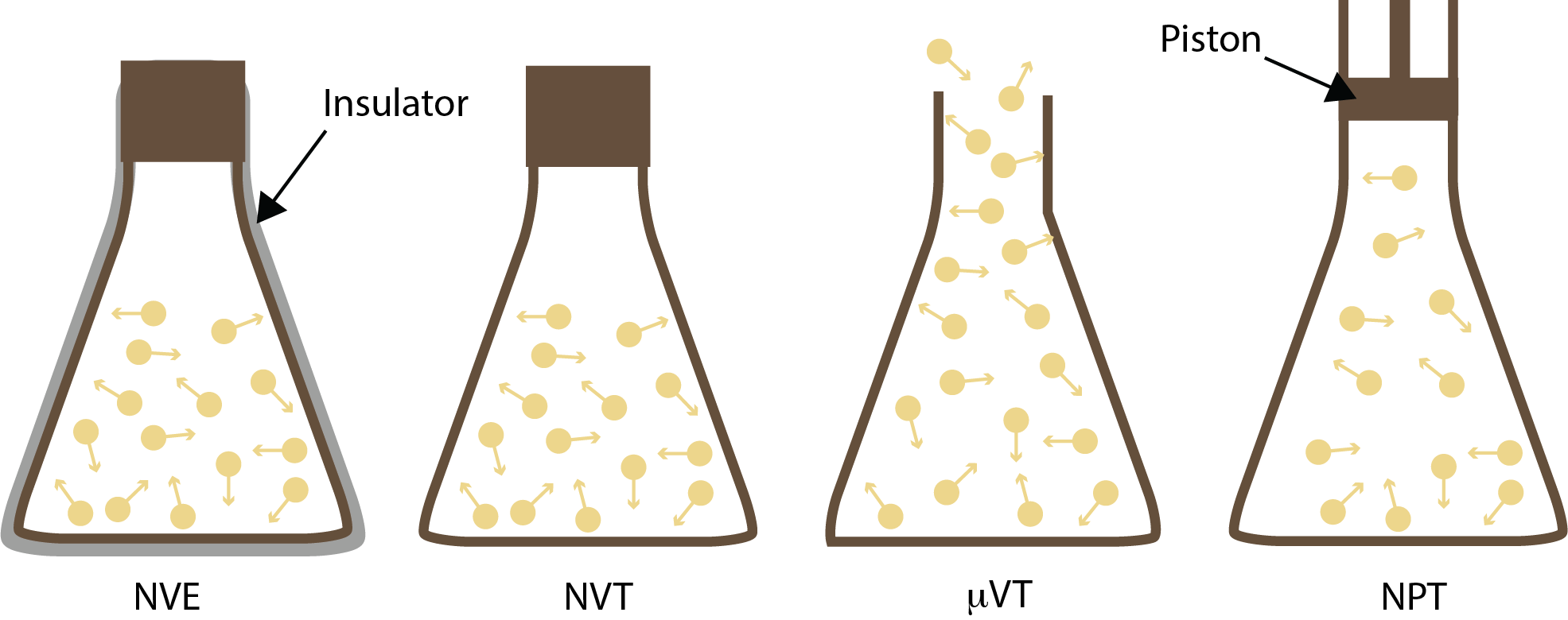
Ensemble is the actual microstates and the probability distribution within the phase space. It is a collection of microstates that share certain macroscopic properties, such as temperature (T), pressure (P), volume (V), number of particles (N). There are several types of ensembles in statistical mechanics, each corresponding to different constraints on the system.

Microcanonical Ensemble (NVE) In the microcanonical ensemble, we consider an isolated system with a fixed number of particles, volume, and energy.

P(E) = \frac{1}{\Omega(E)}

(1)

where $\Omega(E)$ is the number of microstates with energy $E$ . The microcanonical ensemble describes the system’s behavior when it is isolated and not in contact with any external environment.

Canonical Ensemble (NVT) In the canonical ensemble, the system is in thermal equilibrium with a heat bath at a fixed temperature. The number of particles and volume are fixed, but the energy can fluctuate. The probability of each microstate is given by the Boltzmann distribution.

P(E) = \frac{1}{Z}e^{-\beta E}

(2)

Z = \sum e^{-\beta E}

(3)

where $Z$ is the partition function, $\beta = \frac{1}{k_B T}$ is the inverse temperature, and $E$ is the energy of the microstate.

Isothermal-Isobaric Ensemble (NPT) In the isothermal-isobaric ensemble, the system is in thermal and mechanical equilibrium with a heat bath and a pressure bath. The temperature, pressure, and volume are fixed, but the energy and number of particles can fluctuate.

P(E,V) = \frac{1}{Z}e^{-\beta (E+PV)}

(4)

Z = \sum e^{-\beta (E+PV)}

(5)

where $Z$ is the partition function, $P$ is the pressure, and $V$ is the volume of the system.

Grand Canonical Ensemble (μVT) In the grand canonical ensemble, the system is in thermal and chemical equilibrium with a reservoir. The temperature, volume, and chemical potential are fixed, but both the number of particles and the energy can fluctuate, representing an open system where the number of particles can change.

P(E,N) = \frac{1}{Z}e^{-\beta(E-\mu N)}

(6)

Z = \sum e^{-\beta(E-\mu N)}

(7)

where $Z$ is the grand canonical partition function, μ is the chemical potential, and $N$ is the number of particles.

Each ensemble provides a different perspective on the system, allowing for the calculation of macroscopic properties and the understanding of thermodynamic behavior under various constraints.

Thermodynamic Properties¶

Once we know the partition function, we can calculate various thermodynamic properties of the system:

F = -k_B T \ln Z

(8)

U = -\frac{\partial \ln Z}{\partial \beta}=k_B T^2 \frac{\partial \ln Z}{\partial T}

(9)

S = - \frac{\partial F}{\partial T} = k_B \ln Z+k_B T \frac{\partial \ln Z}{\partial T}

(10)

P = -\frac{\partial F}{\partial V}=k_B T \frac{\partial \ln Z}{\partial V}

(11)

H = U + PV = k_B T^2 \frac{\partial \ln Z}{\partial \beta} + k_B T V \frac{\partial \ln Z}{\partial V}

(12)

G = F + PV = -k_B T \ln Z + k_B T V \frac{\partial \ln Z}{\partial V}

(13)

C_v = \frac{\partial U}{\partial T} = k_B \beta^2 \frac{\partial^2 \ln Z}{\partial \beta^2}

(14)

where $F$ is the Helmholtz free energy, $S$ is the entropy, $U$ is the internal energy, $C_v$ is the heat capacity at constant volume, $P$ is the pressure, $V$ is the volume of the system, $H$ is the enthalpy, and $G$ is the Gibbs free energy.

These equations allow us to relate the microscopic properties of the system to its macroscopic behavior and predict how the system will respond to changes in temperature, pressure, and volume.

Sampling the Phase Space¶

One of the main challenges in statistical mechanics is to sample the phase space effectively to obtain accurate statistical averages and thermodynamic properties. Two common methods for sampling the phase space are molecular dynamics and Monte Carlo simulations:

Molecular Dynamics (MD) simulates the motion of particles in the system over time by solving Newton’s equations of motion. By tracking the trajectories of particles, MD provides detailed information about the time evolution of the system and allows for the calculation of time-averaged properties.
Monte Carlo samples the phase space by randomly selecting microstates based on their probabilities. MC simulations use statistical techniques to generate a representative set of microstates, from which ensemble averages can be calculated.

Ergodic hypothesis states that a system will explore all of its microstates over time. According to this hypothesis, the time average of a property of the system is equal to the ensemble average. This implies that by simulating the dynamics of a system for a sufficiently long time, we can obtain accurate statistical averages and thermodynamic properties. Therefore, MD and MC simulation will get the same statistical averages if the system is ergodic and is independent of the initial conditions.

Materials Informatics

Models and Theories II

Materials Informatics

Molecular Dynamics