Monte Carlo
Monte Carlo methods are a class of computational algorithms that rely on random sampling to obtain numerical results. These methods are widely used in various fields, including physics, chemistry, and computer science, to solve complex problems that are difficult or impossible to solve analytically. In atomistic simulation, unlike molecular dynamics (MD), which relies on solving equations of motion for particles over time, Monte Carlo simulations are based on random sampling and statistical sampling methods to explore the configuration space of a system.
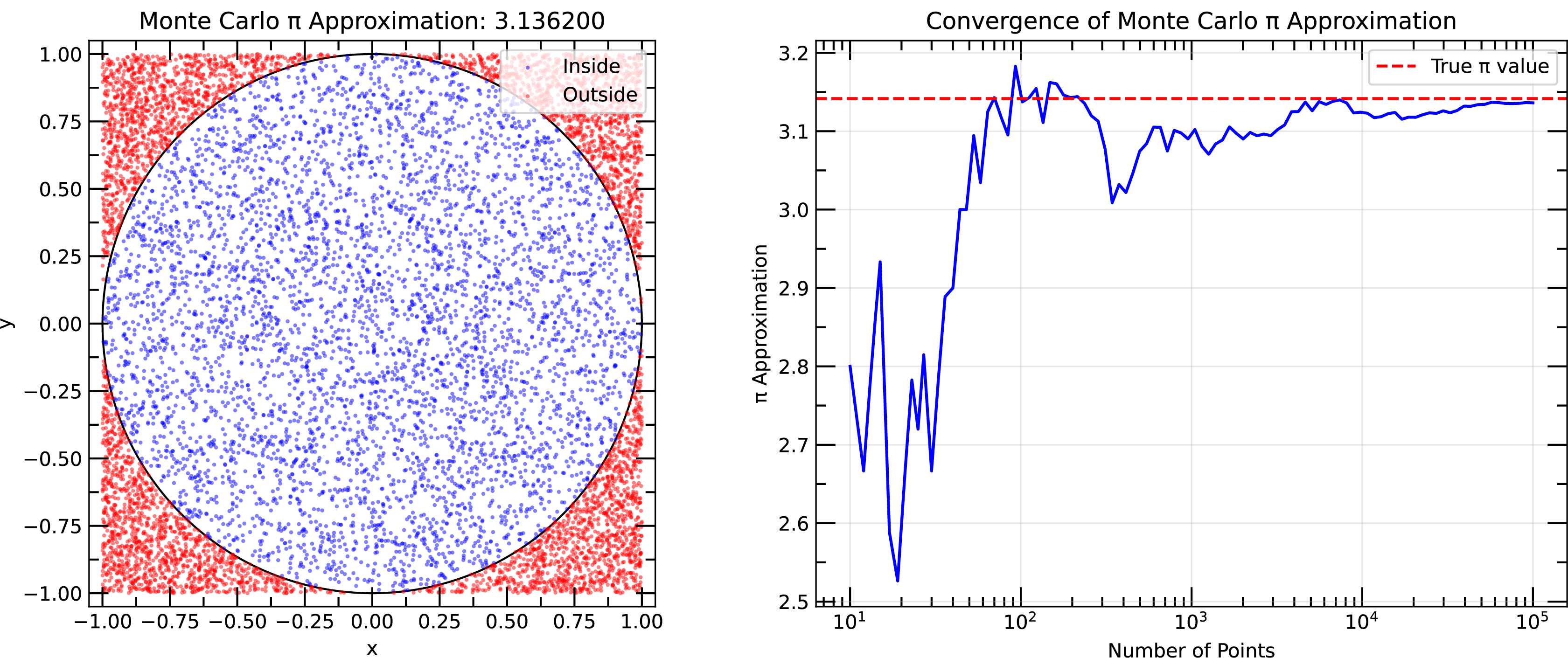
Example of Monte Carlo simulation to estimate the value of using random sampling. Right panel shows the convergence of the estimated value of as a function of the number of samples.
A simple example of a Monte Carlo simulation is the estimation of the value of using random sampling. The idea is to randomly sample points in a square and calculate the fraction of points that fall within a quarter circle inscribed in the square. The ratio of the area of the quarter circle to the area of the square is , so multiplying that sampled fraction by 4 gives an estimate of . By increasing the number of random samples, the estimate of converges to the true value.
Metropolis Algorithm
In principle, you can randomly sample the whole phase space to calculate the properties of a system. However, this is not practical due to the vast number of possible configurations. For example, a system with 100 particles has 10150 possible configurations, which is an astronomically large number. However, most of the configurations have low probability (low Boltzmann factor) and are not relevant to the properties of the system. Therefore, we need a method to sample the phase space effectively to obtain accurate statistical averages and thermodynamic properties.
The Metropolis algorithm is a Monte Carlo method that allows you to sample the phase space effectively by accepting or rejecting proposed moves based on a probability criterion. The Metropolis algorithm is widely used in Monte Carlo simulations to generate a representative set of configurations that can be used to calculate ensemble averages.
The Metropolis algorithm consists of the following steps:
Initialization: Start with an initial configuration of the system.
Propose a Move: Randomly select a particle and propose a move to a new position.
Calculate Energy Change: Calculate the change in energy, , resulting from the proposed move.
Acceptance Criterion: Accept the move with a probability given by the Metropolis criterion:
where is the Boltzmann constant and is the temperature. Energy can be calculated using a force field using the configuration of the system.
Update Configuration: If the move is accepted, update the configuration of the system.
In general, the Metropolis algorithm allows you to explore the configuration space of a system by accepting moves that lower the energy of the system and occasionally accepting moves that increase the energy. With a suitable proposal rule, this stochastic process samples configurations according to their Boltzmann weights and allows you to calculate ensemble averages and thermodynamic properties.
At higher temperatures, the system is more likely to accept moves that increase the energy, allowing it to explore a wider range of configurations. At low temperatures, the system is less likely to accept such moves, leading to a more focused exploration of low-energy configurations.
Applications
Phase Transitions: Monte Carlo simulations are widely used to study phase transitions in various systems, such as the Ising model for magnetic systems and the Lennard-Jones model for fluids.
Protein Folding: Monte Carlo simulations can be used to study the folding pathways of proteins and predict their native structures.
Comparison with Molecular Dynamics
| Feature | Monte Carlo (MC) | Molecular Dynamics (MD) |
|---|---|---|
| Sampling Method | Random sampling | Deterministic integration of equations |
| Time Evolution | No explicit time evolution | Explicit time evolution |
| Efficiency | Efficient for equilibrium properties | Efficient for dynamic properties |
| System Size | Can handle larger systems | Limited by computational cost |
| Temperature Dependence | Can easily simulate different temperatures | Requires separate simulations for each temperature |
| Energy Landscape | Can sometimes escape local minima more easily, depending on the move set | May get trapped in local minima |
| Computational Cost | Generally lower | Generally higher |
| Applications | Equilibrium properties, phase transitions | Dynamic properties, transport phenomena |
| Nonequilibrium Processes | Not naturally time-accurate for dynamical nonequilibrium processes | Can simulate nonequilibrium processes |