Force Fields
In atomistic modelling, force fields are used to describe the interactions between atoms and molecules in materials. Force fields are mathematical models that represent the potential energy surface of a system, which describes the energy of the system as a function of the atomic positions, and can be used to predict the structure, dynamics, and properties of materials.
Force fields usually contains parameters that describe the interactions between atoms or molecules, such as bond lengths, bond angles, dihedral angles, and non-bonded interactions. These parameters are usually derived from experimental data or quantum mechanical calculations, and are used to fit the force field to reproduce the properties of the material.
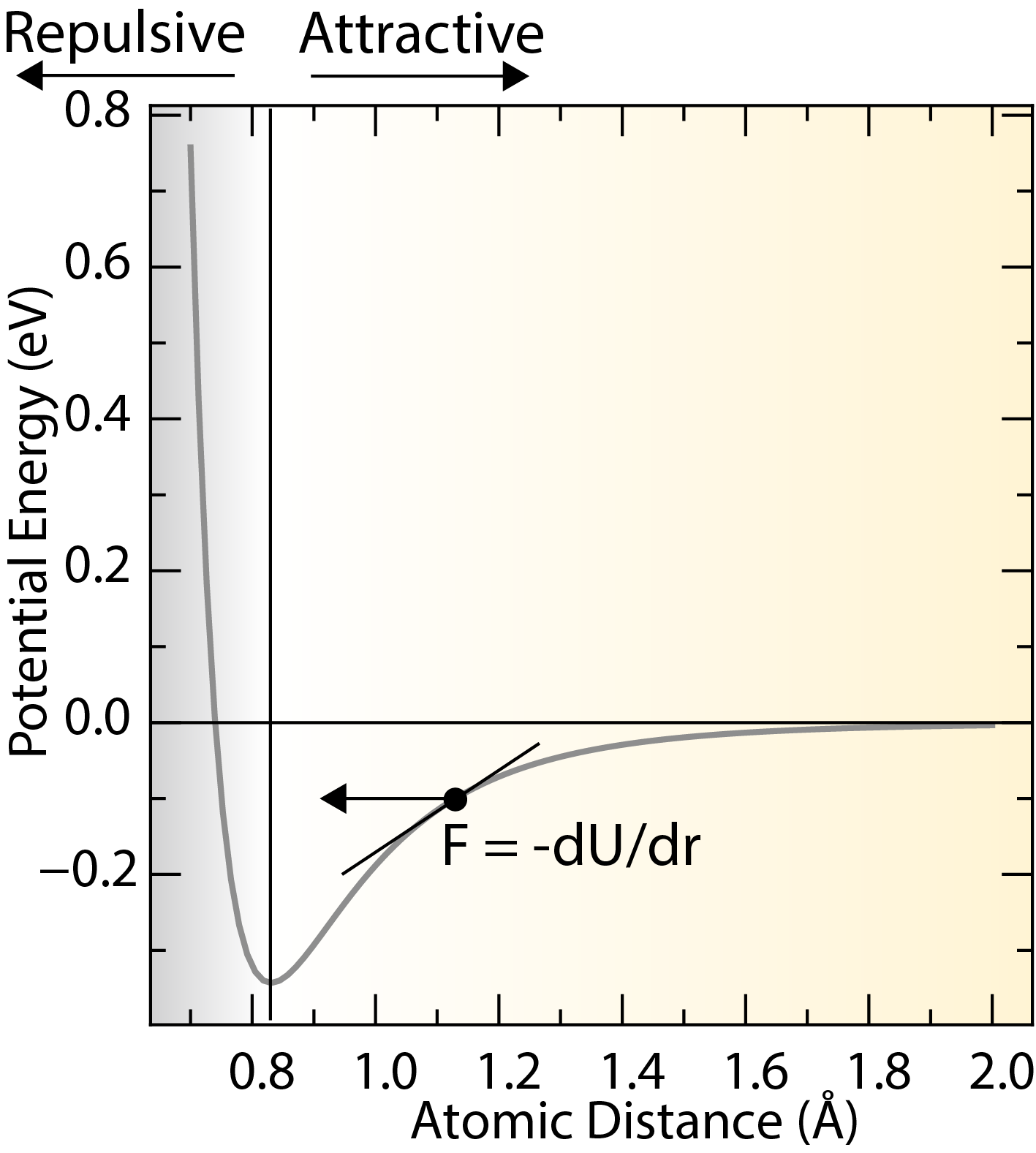
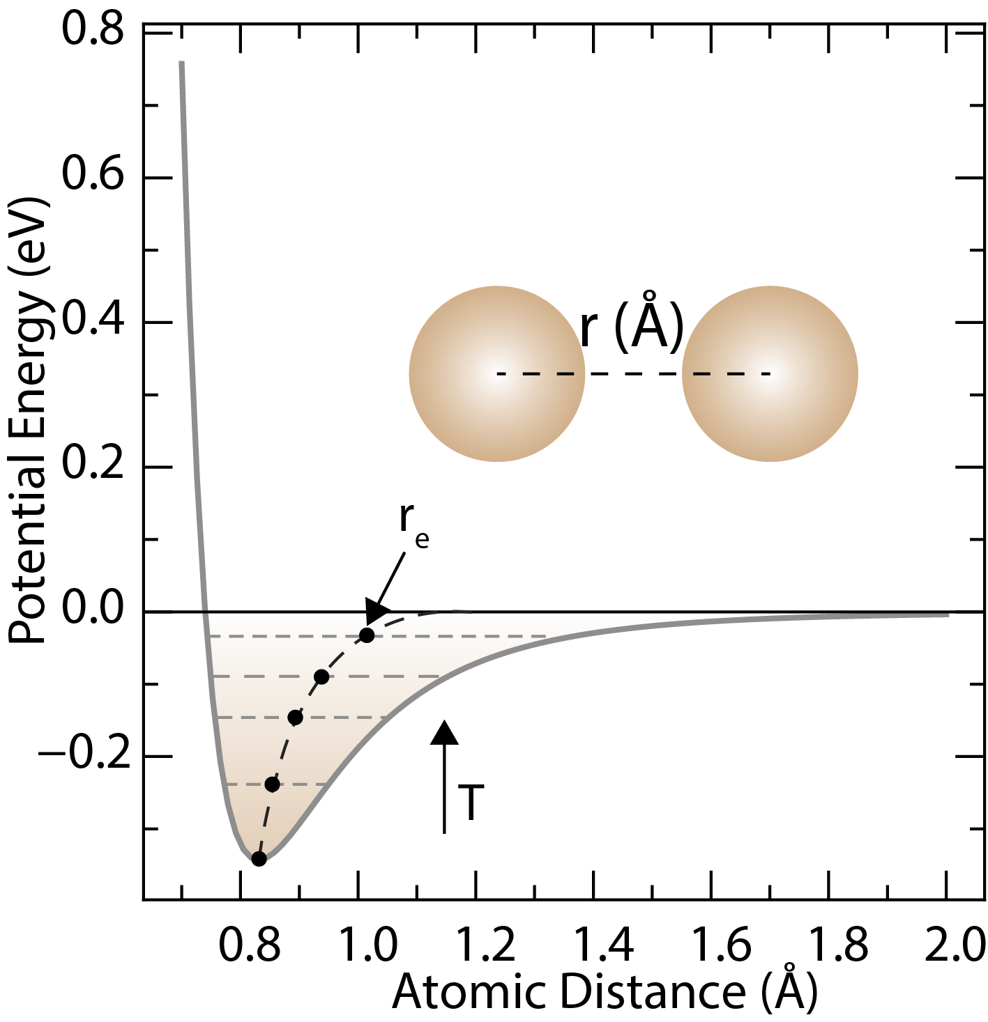
A typical potential energy curves for a pair of atoms as a function of the separation distance.
The center of force fields is the potential energy function (), which describes the interactions between atoms or molecules in a material. The potential energy function is usually expressed as a sum of interactions between atoms or molecules, and can include terms that describe bond stretching, bond bending, torsion, and non-bonded interactions.
where is the energy associated with bond stretching, is the energy associated with bond bending, is the energy associated with torsion. and are usually approximated under the harmonic approximation. is the energy associated with non-bonded interactions such as van der Waals forces and electrostatic interactions.
Interatomic Forces
Interatomic forces can be derived from the potential energy function by taking the negative gradient of the potential energy with respect to the atomic positions.
For solid materials, the stress tensor is obtained from the derivative of the potential energy with respect to strain (or, equivalently, from the virial expression), not from derivatives with respect to atomic positions.
Computational Cost
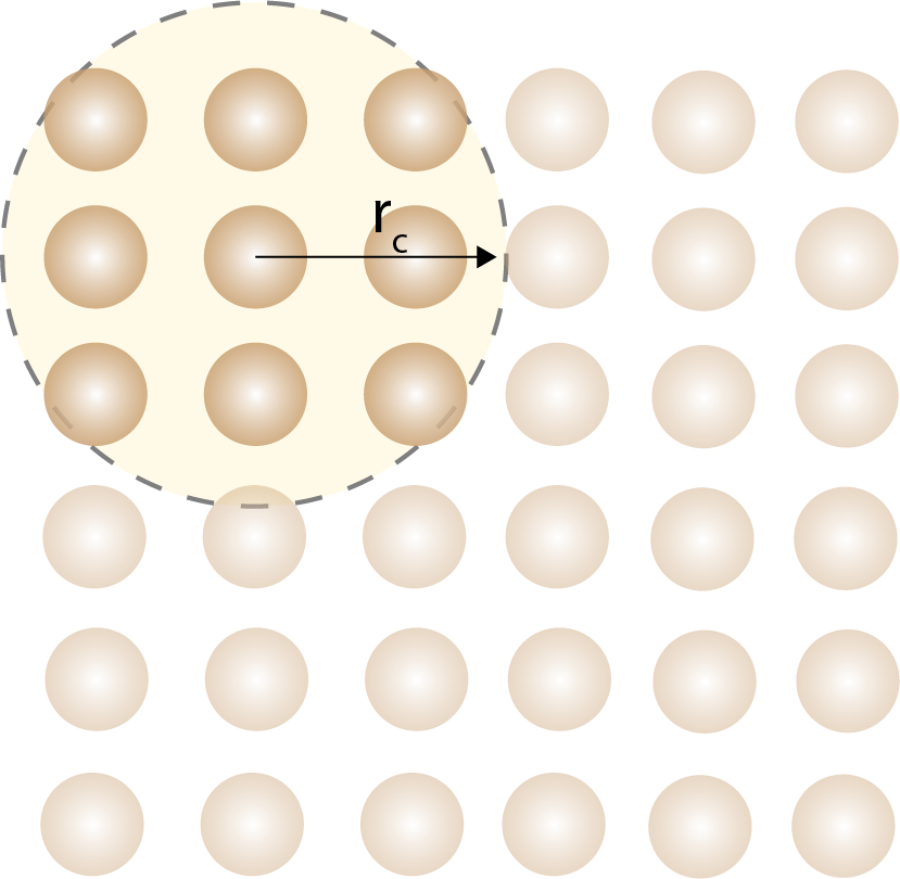
A cutoff distance is used to limit the number of interactions that need to be calculated in force fields.
The computational cost of force fields depends on the number of atoms in the system and the number of interactions that need to be calculated. For short-ranged interactions with cutoffs and neighbor lists, the cost can scale approximately linearly with the number of atoms. Most interactions in force fields are short-ranged, which means that the interactions between atoms decay rapidly with distance. This allows us to use cutoff distances to limit the number of interactions that need to be calculated. The short-range interactions are only evaluated for atoms in the neighbor list, which is usually a small fraction of the total number of atoms. The long-range interactions are more tricky to calculate and are usually the bottleneck of computations. Methods such as Ewald summation are used to calculate long-range electrostatic interactions.
In practice, the unit cell is divided into a grid, and the atoms are assigned to grid cells. The interactions between atoms are calculated only for atoms in the same or neighboring grid cells. This reduces the number of interactions that need to be calculated and improves the efficiency of the simulation.
Periodic Boundary Conditions
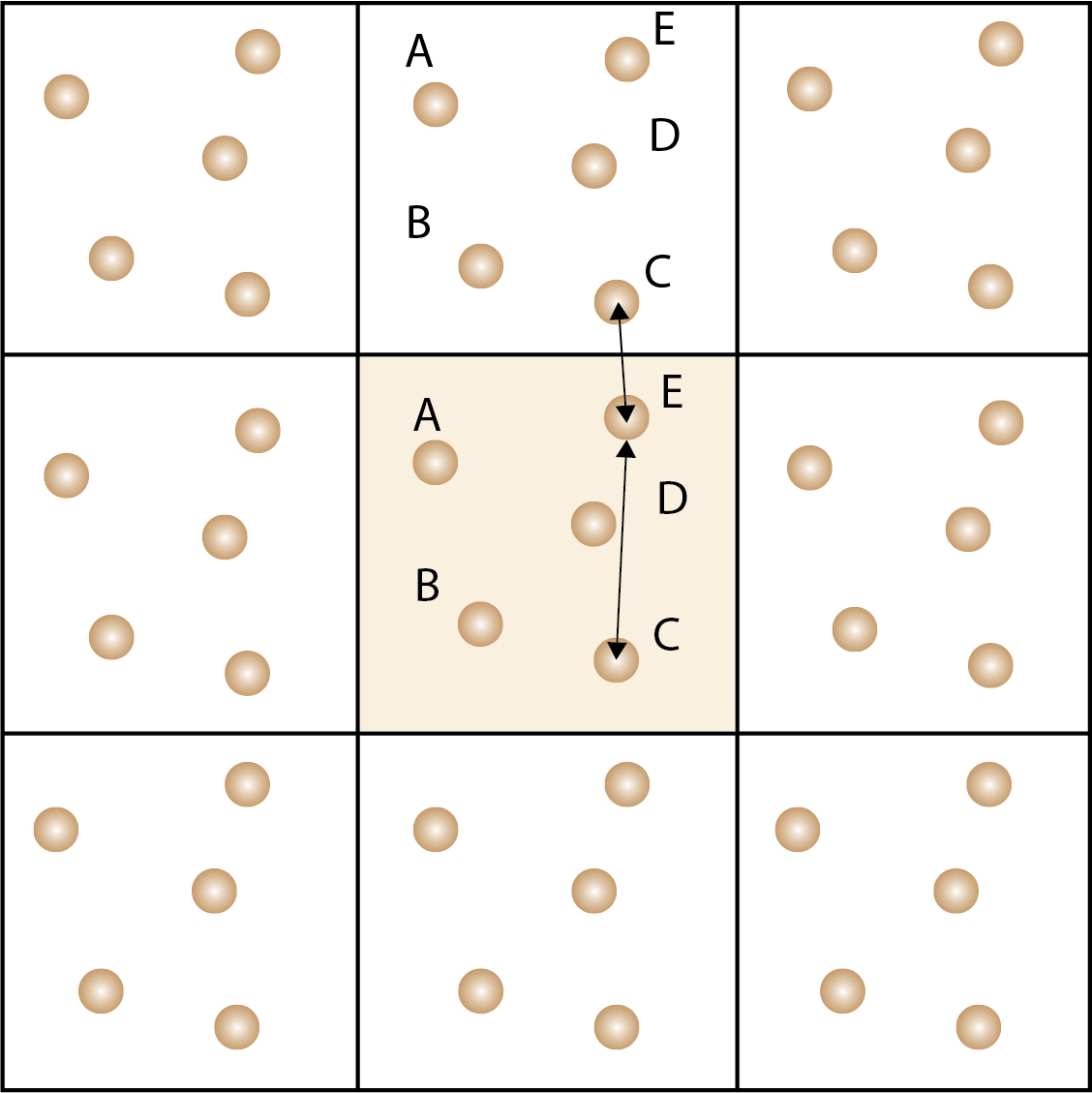
Periodic boundary conditions are used to simulate an infinite system by replicating the simulation cell in all directions. Atoms that leave the simulation cell re-enter from the opposite side. Minimal image convention is used to calculate the distance between atoms in the simulation cell and the neighboring cells.
In solid state materials, the structure has translational symmetry, which means that we can apply a periodic boundary condition to the simulation cell to mimic an infinite system. Mathematically, the periodic boundary condition is applied by replicating the simulation cell in all directions, so that atoms that leave the simulation cell re-enter (wrap) from the opposite side. This allows us to simulate the dynamics of the system without the need to model an infinite system. For a cubic cell with side length :
where is the wrapped position of the atom, is the position of the atom in the simulation cell, is the side length of the cubic simulation cell, and is the rounding function.
The wrapped distance between atoms in the simulation cell and the neighboring cells:
where is the minimum-image displacement vector between atoms and , and are the positions of atoms and , and is the side length of the cubic simulation cell.
Molecular Mechanics Force Fields
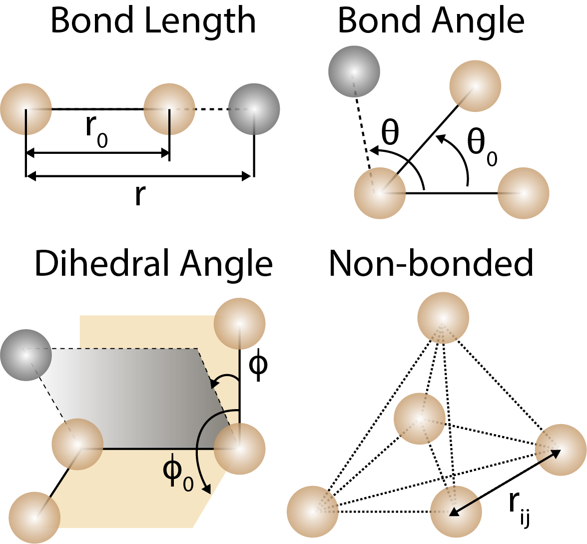
Bond lengths, bond angles, and dihedral angles are used to describe the geometry of molecules in force fields. Non-bonded interactions are used to describe the interactions between atoms that are not directly bonded.
Below are some common force fields terms used in molecular mechanics simulations:
where , , and are the force constants for bond stretching, bond bending, and torsion, is the bond length, is the bond angle, is the dihedral angle, , , and are the equilibrium bond length, bond angle, and dihedral angle, is the multiplicity of the dihedral angle, is the phase shift of the dihedral angle, is the distance between atoms and , is the Lennard-Jones potential, and is the electrostatic potential. Examples of common force fields include CHARMM, AMBER, and GROMOS.
Ewald Summation
The electrostatic potential energy term in the potential energy function is long-ranged and can be difficult to calculate accurately in periodic systems. The Ewald summation is a method for calculating the electrostatic potential energy between charged particles in a periodic system. The Ewald summation is based on the idea of splitting the electrostatic potential into short-range and long-range components, and calculating each component separately.
The short-range component is calculated using a real-space sum, while the long-range component is calculated using a reciprocal-space sum.
The short-range component is calculated in real space and converges rapidly. In atomic units, a common expression is:
where and are the charges of atoms and , is the Ewald parameter, is the distance between atoms and , and is the complementary error function, . The parameter controls how much of the interaction is treated in real space versus reciprocal space: smaller gives a longer-ranged real-space sum, while larger shifts more of the work to reciprocal space.
The long-range component is calculated using the following equation:
where is a reciprocal lattice vector, is the volume of the simulation cell, is the Ewald parameter, is the charge of atom , and is the position of atom . In standard Ewald summation, the reciprocal-space sum is evaluated explicitly and is more expensive than short-range interactions. Mesh-based variants such as particle-mesh Ewald (PME) or PPPM use FFTs and can reduce the scaling to approximately .
The self-interaction term is calculated using the following equation:
where is the Ewald parameter and is the charge of atom . This term removes the unphysical interaction of each charge with its own smeared Gaussian charge distribution.
Pair Potentials
Pair potentials are a type of force field that describes the interactions between pairs of atoms or molecules in a material. Pair potentials are based on the assumption that the interactions between atoms or molecules can be approximated as pairwise interactions, where the potential energy between two atoms or molecules depends only on their separation distance.
Lennard-Jones Potential
The Lennard-Jones potential describes the interactions between neutral atoms or molecules. The depth of the potential well is , is the distance at which the potential crosses zero, and the equilibrium separation is .
Lennard-Jones potential is a simple mathematical model that describes the interactions between neutral atoms or molecules. The Lennard-Jones potential is given by the following equation:
where is the potential energy between two atoms or molecules at a distance , is the depth of the potential well, and is the distance at which the potential energy is zero.
12 and 6 are the powers of the terms in the equation, which represent the repulsive and attractive forces between the atoms or molecules, respectively. The repulsive term accounts for the Pauli exclusion principle, which prevents atoms or molecules from occupying the same space, while the attractive term accounts for the van der Waals forces between the atoms or molecules.
Morse Potential
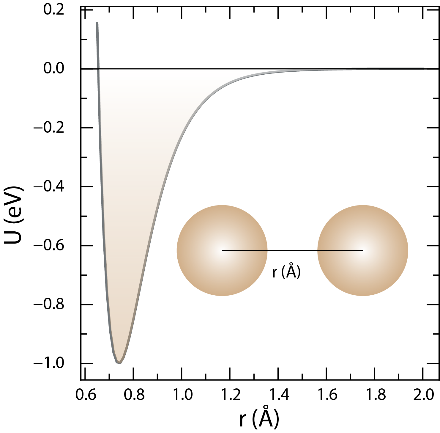
The Morse potential describes the interactions between atoms or molecules in a material. The dissociation energy is , the width of the potential well is , and the equilibrium bond length is .
Morse potential is another mathematical model that describes the interactions between atoms or molecules. The Morse potential is given by the following equation:
where is the potential energy between two atoms or molecules at a distance , is the dissociation energy of the bond, is the width of the potential well, and is the equilibrium bond length.
Many Body Expansion
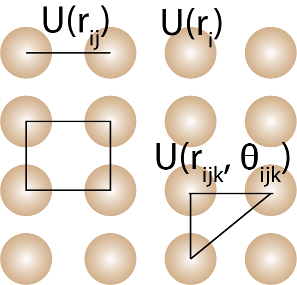
Many-body potentials describe the interactions between three or more atoms or molecules in a material. The many-body expansion includes one-body, two-body, three-body, and higher-order terms that describe the interactions between atoms or molecules.
The potential energy function can be expanded into many-body terms that describe the interactions between three or more atoms or molecules in a material. The many-body expansion is a decomposition of the total energy into one-body, two-body, three-body, and higher-order contributions. The expansion is given by the following equation:
where is the potential energy of atom , is the potential energy between atoms and , is the potential energy between atoms , , and , and so on. is the angle between atoms , , and . The one-body term is only meaningful if atoms are in an external field and is usually ignored in most force fields.
Many-body potentials are a type of force field that describes the interactions between three or more atoms or molecules in a material. Many-body potentials are used to capture the effects of many-body interactions, such as bond bending, torsion, and non-bonded interactions, which cannot be described by pair potentials alone.
Tersoff Potential
Tersoff potential (bond order potentials) is a many-body potential that describes the interactions between atoms in covalently bonded materials. The Tersoff potential is given by the following equation:
where is the potential energy of the system, is the cutoff function that determines the range of the potential, is the repulsive term that accounts for short-range core repulsion, is the bonding term, is the bond-order term that describes how the bond strength between atoms and depends on the local environment, and is the distance between atoms and . The bond-order term is a function of the bond length, bond angle, and coordination number of the atoms, which gives the potential its many-body character.
Embedded Atom Method (EAM)
Embedded Atom Method (EAM) is another many-body potential that describes the interactions between atoms in metallic materials. The EAM potential is based on the assumption that the energy of an atom in a material is a function of the electron density around the atom. The EAM potential is given by the following equation:
where is the total energy of the system, is the embedding energy of atom , is the electron density around atom , is the pair potential energy between atoms and at a distance .
Other similar potentials: effective medium theory (EMT) and modified embedded atom method (MEAM).
Other Force Fields
There are many other types of force fields and potentials that are used in atomistic modelling, depending on the specific properties of the material being studied. Some examples include: reactive force fields, polarizable force fields, and coarse-grained force fields.
Recently, machine learning potentials have gained popularity in materials science, where machine learning algorithms are used to develop force fields that can accurately predict the properties of materials without the need for explicit parameterization.
where is the machine learning potential, is the machine learning model, and is the descriptor of the system, such as the atomic positions, charges, and forces. A more detailed discussion of machine learning potentials will be covered in the later lectures.