Pandas Basics
Pandas is a powerful Python library for data manipulation and analysis. In materials informatics, Pandas is commonly used to work with data from databases like the Materials Project, analyze simulation results, and prepare data for visualization.
Introduction to Pandas
Pandas provides two main data structures:
Series: A one-dimensional labeled array (like a column in a spreadsheet)
DataFrame: A two-dimensional labeled data structure (like a spreadsheet or SQL table)
DataFrames are the most commonly used structure and will be used throughout this course for handling materials data.
Creating DataFrames
There are several ways to create DataFrames. The most common way is from dictionaries.
import pandas as pd
import numpy as np

# Create a DataFrame from a dictionary
data = {
    'material_id': ['mp-1', 'mp-2', 'mp-3', 'mp-4', 'mp-5'],
    'density': [5.2, 3.1, 4.8, 2.9, 5.5],
    'bulk_modulus': [150, 120, 180, 110, 160],
    'shear_modulus': [80, 70, 95, 60, 85]
}

df = pd.DataFrame(data)
print(df)
material_id density bulk_modulus shear_modulus
0 mp-1 5.2 150 80
1 mp-2 3.1 120 70
2 mp-3 4.8 180 95
3 mp-4 2.9 110 60
4 mp-5 5.5 160 85
# Display first 5 rows
print("First rows:")
print(df.head())
# Display last 5 rows
print("\nLast rows:")
print(df.tail())
# Display summary statistics
print("\nSummary statistics:")
print(df.describe())
# Display DataFrame shape (rows, columns)
print(f"\nDataFrame shape: {df.shape}")First rows:
  material_id  density  bulk_modulus  shear_modulus
0        mp-1      5.2           150             80
1        mp-2      3.1           120             70
2        mp-3      4.8           180             95
3        mp-4      2.9           110             60
4        mp-5      5.5           160             85
Last rows:
material_id density bulk_modulus shear_modulus
0 mp-1 5.2 150 80
1 mp-2 3.1 120 70
2 mp-3 4.8 180 95
3 mp-4 2.9 110 60
4 mp-5 5.5 160 85
Summary statistics:
density bulk_modulus shear_modulus
count 5.000000 5.000000 5.000000
mean 4.300000 144.000000 78.000000
std 1.214496 28.809721 13.509256
min 2.900000 110.000000 60.000000
25% 3.100000 120.000000 70.000000
50% 4.800000 150.000000 80.000000
75% 5.200000 160.000000 85.000000
max 5.500000 180.000000 95.000000
DataFrame shape: (5, 4)
Selecting Data
# Select single column (returns a Series)
material_ids = df['material_id']
print("Single column:")
print(material_ids)

# Select multiple columns (returns a DataFrame)
print("\nMultiple columns:")
subset = df[['material_id', 'density']]
print(subset)

# Select rows by index
print("\nFirst 3 rows:")
first_3 = df.iloc[0:3]
print(first_3)

# Select rows by condition
print("\nMaterials with density > 4.0:")
high_density = df[df['density'] > 4.0]
print(high_density)

# Select rows with multiple conditions
print("\nMaterials with density between 3 and 5:")
medium_density = df[(df['density'] >= 3.0) & (df['density'] <= 5.0)]
print(medium_density)
Single column:
0 mp-1
1 mp-2
2 mp-3
3 mp-4
4 mp-5
Name: material_id, dtype: str
Multiple columns:
material_id density
0 mp-1 5.2
1 mp-2 3.1
2 mp-3 4.8
3 mp-4 2.9
4 mp-5 5.5
First 3 rows:
material_id density bulk_modulus shear_modulus
0 mp-1 5.2 150 80
1 mp-2 3.1 120 70
2 mp-3 4.8 180 95
Materials with density > 4.0:
material_id density bulk_modulus shear_modulus
0 mp-1 5.2 150 80
2 mp-3 4.8 180 95
4 mp-5 5.5 160 85
Materials with density between 3 and 5:
material_id density bulk_modulus shear_modulus
1 mp-2 3.1 120 70
2 mp-3 4.8 180 95
Basic Aggregation and Statistics
# Calculate mean of a column
mean_density = df['density'].mean()
print(f"Mean density: {mean_density:.2f}")

# Calculate standard deviation
std_density = df['density'].std()
print(f"Std dev density: {std_density:.2f}")

# Find minimum and maximum
min_bulk = df['bulk_modulus'].min()
max_bulk = df['bulk_modulus'].max()
print(f"Bulk modulus range: {min_bulk} - {max_bulk} GPa")

# Sum of values
total_shear = df['shear_modulus'].sum()
print(f"Total shear modulus: {total_shear} GPa")

# Count of non-null values
count = df['bulk_modulus'].count()
print(f"Count of bulk modulus values: {count}")

# Median
median_density = df['density'].median()
print(f"Median density: {median_density:.2f}")
Mean density: 4.30
Std dev density: 1.21
Bulk modulus range: 110 - 180 GPa
Total shear modulus: 390 GPa
Count of bulk modulus values: 5
Median density: 4.80
Filtering and Sorting
# Sort by column (ascending)
print("Sorted by density (ascending):")
df_sorted = df.sort_values('density')
print(df_sorted)

# Sort by column (descending)
print("\nSorted by density (descending):")
df_sorted_desc = df.sort_values('density', ascending=False)
print(df_sorted_desc)

# Sort by multiple columns
print("\nSorted by bulk modulus then density:")
df_multi_sort = df.sort_values(['bulk_modulus', 'density'])
print(df_multi_sort)
Sorted by density (ascending):
material_id density bulk_modulus shear_modulus
3 mp-4 2.9 110 60
1 mp-2 3.1 120 70
2 mp-3 4.8 180 95
0 mp-1 5.2 150 80
4 mp-5 5.5 160 85
Sorted by density (descending):
material_id density bulk_modulus shear_modulus
4 mp-5 5.5 160 85
0 mp-1 5.2 150 80
2 mp-3 4.8 180 95
1 mp-2 3.1 120 70
3 mp-4 2.9 110 60
Sorted by bulk modulus then density:
material_id density bulk_modulus shear_modulus
3 mp-4 2.9 110 60
1 mp-2 3.1 120 70
0 mp-1 5.2 150 80
4 mp-5 5.5 160 85
2 mp-3 4.8 180 95
# Add new column (e.g., bulk/shear ratio)
df['bulk_shear_ratio'] = df['bulk_modulus'] / df['shear_modulus']
print("DataFrame with new column:")
print(df)

# Remove column
df_copy = df.copy()
df_copy = df_copy.drop('bulk_shear_ratio', axis=1)
print("\nAfter dropping bulk_shear_ratio:")
print(df_copy)
DataFrame with new column:
material_id density bulk_modulus shear_modulus bulk_shear_ratio
0 mp-1 5.2 150 80 1.875000
1 mp-2 3.1 120 70 1.714286
2 mp-3 4.8 180 95 1.894737
3 mp-4 2.9 110 60 1.833333
4 mp-5 5.5 160 85 1.882353
After dropping bulk_shear_ratio:
material_id density bulk_modulus shear_modulus
0 mp-1 5.2 150 80
1 mp-2 3.1 120 70
2 mp-3 4.8 180 95
3 mp-4 2.9 110 60
4 mp-5 5.5 160 85
Renaming Columns
# Rename single column
df_renamed = df.rename(columns={'material_id': 'mp_id'})
print("After renaming material_id to mp_id:")
print(df_renamed.head())

# Rename multiple columns
df_renamed_multi = df.rename(columns={
    'bulk_modulus': 'bulk_modulus_GPa',
    'shear_modulus': 'shear_modulus_GPa'
})
print("\nAfter renaming modulus columns:")
print(df_renamed_multi.head())
After renaming material_id to mp_id:
mp_id density bulk_modulus shear_modulus bulk_shear_ratio
0 mp-1 5.2 150 80 1.875000
1 mp-2 3.1 120 70 1.714286
2 mp-3 4.8 180 95 1.894737
3 mp-4 2.9 110 60 1.833333
4 mp-5 5.5 160 85 1.882353
After renaming modulus columns:
material_id density bulk_modulus_GPa shear_modulus_GPa bulk_shear_ratio
0 mp-1 5.2 150 80 1.875000
1 mp-2 3.1 120 70 1.714286
2 mp-3 4.8 180 95 1.894737
3 mp-4 2.9 110 60 1.833333
4 mp-5 5.5 160 85 1.882353
Handling Missing Values
# Create a DataFrame with missing values
data_missing = {
    'material_id': ['mp-1', 'mp-2', 'mp-3', 'mp-4', 'mp-5'],
    'density': [5.2, np.nan, 4.8, 2.9, np.nan],
    'bulk_modulus': [150, 120, np.nan, 110, 160]
}

df_missing = pd.DataFrame(data_missing)
print("DataFrame with missing values:")
print(df_missing)

# Check for missing values
print("\nMissing values count:")
print(df_missing.isnull().sum())

# Drop rows with missing values
print("\nAfter dropping rows with missing values:")
df_clean = df_missing.dropna()
print(df_clean)

# Fill missing values with mean
print("\nAfter filling missing values with mean:")
numeric_means = df_missing.mean(numeric_only=True)
df_filled = df_missing.fillna(numeric_means)
print(df_filled)
DataFrame with missing values:
material_id density bulk_modulus
0 mp-1 5.2 150.0
1 mp-2 NaN 120.0
2 mp-3 4.8 NaN
3 mp-4 2.9 110.0
4 mp-5 NaN 160.0
Missing values count:
material_id 0
density 2
bulk_modulus 1
dtype: int64
After dropping rows with missing values:
material_id density bulk_modulus
0 mp-1 5.2 150.0
3 mp-4 2.9 110.0
After filling missing values with mean:
material_id density bulk_modulus
0 mp-1 5.2 150.0
1 mp-2 4.3 120.0
2 mp-3 4.8 135.0
3 mp-4 2.9 110.0
4 mp-5 4.3 160.0
Integration with Matplotlib
Pandas integrates seamlessly with Matplotlib for plotting.
import matplotlib.pyplot as plt

# Scatter plot
plt.figure(figsize=(8, 6))
plt.scatter(df['density'], df['bulk_modulus'], alpha=0.6, s=100, color='blue')
plt.xlabel('Density (g cm$^{-3}$)', fontsize=12)
plt.ylabel('Bulk Modulus (GPa)', fontsize=12)
plt.title('Bulk Modulus vs Density', fontsize=14)
plt.grid(True, alpha=0.3)
plt.show()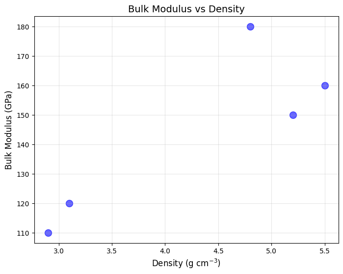
# Histogram
plt.figure(figsize=(8, 6))
plt.hist(df['density'], bins=10, edgecolor='black', color='green', alpha=0.7)
plt.xlabel('Density (g cm$^{-3}$)', fontsize=12)
plt.ylabel('Frequency', fontsize=12)
plt.title('Distribution of Density Values', fontsize=14)
plt.grid(True, alpha=0.3, axis='y')
plt.show()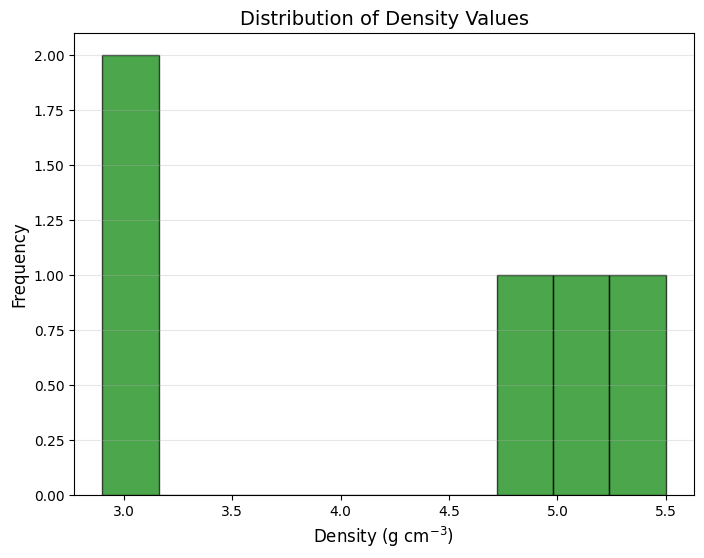
# Plot bulk and shear modulus vs density
plt.figure(figsize=(8, 6))
plt.scatter(df['density'], df['bulk_modulus'], label='Bulk Modulus', alpha=0.6, s=100)
plt.scatter(df['density'], df['shear_modulus'], label='Shear Modulus', alpha=0.6, s=100)
plt.xlabel('Density (g cm$^{-3}$)', fontsize=12)
plt.ylabel('Modulus (GPa)', fontsize=12)
plt.title('Bulk and Shear Modulus vs Density', fontsize=14)
plt.legend(fontsize=10)
plt.grid(True, alpha=0.3)
plt.show()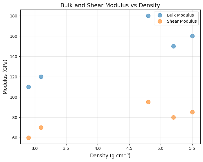
# Save our current DataFrame to CSV
df.to_csv('materials_data.csv', index=False)
print("Saved to materials_data.csv")

# Read it back
df_loaded = pd.read_csv('materials_data.csv')
print("\nLoaded from CSV:")
print(df_loaded.head())
Saved to materials_data.csv
Loaded from CSV:
material_id density bulk_modulus shear_modulus bulk_shear_ratio
0 mp-1 5.2 150 80 1.875000
1 mp-2 3.1 120 70 1.714286
2 mp-3 4.8 180 95 1.894737
3 mp-4 2.9 110 60 1.833333
4 mp-5 5.5 160 85 1.882353
Common file formats you can read/write:
| Format | Read Function | Write Function | Example |
|---|---|---|---|
| CSV | pd.read_csv() | df.to_csv() | df = pd.read_csv('data.csv') |
| JSON | pd.read_json() | df.to_json() | df = pd.read_json('data.json') |
| Excel | pd.read_excel() | df.to_excel() | df = pd.read_excel('data.xlsx') |
| TSV | pd.read_csv() with sep='\t' | df.to_csv() with sep='\t' | df = pd.read_csv('data.tsv', sep='\t') |
| HDF5 | pd.read_hdf() | df.to_hdf() | df = pd.read_hdf('data.h5', key='table') |
HDF5 (Hierarchical Data Format)
HDF5 is useful for large, structured datasets and fast I/O. Pandas uses PyTables under the hood.
You need to run following in Terminal after activating your venv.
pip3 install tables h5py# Save to HDF5 (requires PyTables)
hdf5_path = 'materials_data.h5'
df.to_hdf(hdf5_path, key='materials', mode='w')
print(f"Saved to {hdf5_path}")
# Read back from HDF5
df_hdf = pd.read_hdf(hdf5_path, key='materials')
print("\nLoaded from HDF5:")
print(df_hdf.head())Saved to materials_data.h5
Loaded from HDF5:
material_id density bulk_modulus shear_modulus bulk_shear_ratio
0 mp-1 5.2 150 80 1.875000
1 mp-2 3.1 120 70 1.714286
2 mp-3 4.8 180 95 1.894737
3 mp-4 2.9 110 60 1.833333
4 mp-5 5.5 160 85 1.882353
Performance Tips
When working with large datasets:
Use vectorized operations instead of loops whenever possible
Use
df.iloc[]for integer location-based indexing (faster thandf.loc[])Use
inplace=Trueto modify DataFrame in place (saves memory)Specify
dtypewhen reading files to reduce memory usageUse
.copy()when you need to work with a separate copy of the data
# Example: Vectorized operation vs loop
# Vectorized (FAST)
df['bulk_shear_ratio_fast'] = df['bulk_modulus'] / df['shear_modulus']

# Loop (SLOW - don't do this for large datasets!)
df['bulk_shear_ratio_slow'] = 0.0
for i in range(len(df)):
    df.loc[i, 'bulk_shear_ratio_slow'] = df.loc[i, 'bulk_modulus'] / df.loc[i, 'shear_modulus']

# Verify they're the same
print("Vectorized and loop methods give same result:")
print(df[['bulk_shear_ratio_fast', 'bulk_shear_ratio_slow']])
Vectorized and loop methods give same result:
bulk_shear_ratio_fast bulk_shear_ratio_slow
0 1.875000 1.875000
1 1.714286 1.714286
2 1.894737 1.894737
3 1.833333 1.833333
4 1.882353 1.882353
Summary
Key Pandas operations you’ll use in this section:
| Operation | Description | Example |
|---|---|---|
| Creating | Create from dictionary | df = pd.DataFrame(data) |
| Loading | Read CSV/JSON files | df = pd.read_csv('data.csv') |
| Selecting | Access columns/rows | df['col'] or df[df['col'] > 5] |
| Filtering | Select rows based on conditions | df[df['density'] > 4.0] |
| Aggregation | Calculate statistics | df['col'].mean(), df.describe() |
| Adding columns | Create new derived data | df['new_col'] = df['col1'] / df['col2'] |
| Plotting | Visualize with Matplotlib | plt.scatter(df['x'], df['y']) |
| Saving | Write to file | df.to_csv('output.csv') |