Practical: Python Programming using VS Code and Jupyter Notebook

This practical will guide you through basics of Python programming language and Jupyter notebook using VS Code. Please make sure you have setup your environment correctly before starting the practical.

Write a Simple Python Code¶

Python will be the primary programming language used in this course.

Create a folder on your desktop and name it materials_informatics. Open this folder using VS Code by clicking File -> Open Folder and selecting the folder (materials_informatics) you just created.

On the left panel in Folders, right click and select New File named hello_world.py. Open the file using VS Code and write the following code:

print("Hello, World!")

Make sure you have select the correct Python interpreter to take the advantage of features such as syntax highlighting, code completion and debugging.

Python scripts are executed using an interpreter, which can be done by running the command:

python hello_world.py

You should see the output Hello, World! printed on the terminal.

Since most of the student already know some basic Python, we won’t treat everybody as the absolute beginner. There are lots of online resources to learn Python and you can choose any of them. For introductory videos on Python, please refer to the following link: Introductory Videos on Python provided by Dr. Sasani Jayawardhana.

Jupyter Notebook¶

Jupyter Notebook is an open-source interactive tool widely used in programming and data science. It provides a web-based interface that allows you to create and share documents containing live code, equations, visualizations, and narrative text.

One of the key features of Jupyter Notebooks is interactive coding. This feature allows you to run code incrementally, making it an excellent tool for testing and debugging. Additionally, Jupyter Notebooks support rich content, enabling you to include various types of content such as text, images, videos, and interactive visualizations. This makes it ideal for data visualization and exploratory data analysis.

The interface of Jupyter Notebooks supports both code cells and markdown cells. Code cells allow you to write and execute code, while markdown cells enable you to write formatted text. This combination of code and narrative text in a single document enhances the readability and comprehensibility of your work.

Furthermore, Jupyter Notebooks can be integrated with Visual Studio Code using the Jupyter plugin. This integration provides a seamless coding experience, allowing you to leverage the powerful features of VS Code while working with Jupyter Notebooks.

By leveraging Jupyter Notebooks, you can create comprehensive and interactive documents that enhance your programming and data analysis workflows.

Creating a New Jupyter Notebook in VS Code¶

Open Visual Studio Code.
Ensure you have the Jupyter extension installed. If not, you can install it from the Extensions view (Ctrl/Command+Shift+X). Also make sure you have installed the Jupyter package package in your virtual environment.
Open the Command Palette (Ctrl+Shift+P) and type Create: New Jupyter Notebook.
Click Select Kernel, then Python Environments, and choose the interpreter in your created virtual environment, e.g. mi (Python 3.13.1).
A new Jupyter Notebook will be created, and you can start adding code and markdown cells as needed.
You should save it as a file with extension of .ipynb, e.g. wk01.ipynb.

By following these steps, you can create a new Jupyter Notebook in VS Code and begin your interactive coding and data analysis tasks.

Markdown¶

Markdown is a lightweight markup language with plain text formatting syntax. It is widely used for creating formatted text using a plain-text editor. In this course, Markdown will be used for documentation purposes. Files written in Markdown typically have the .md extension. You can also write markdown in the Markdown cell of a Jupyter Notebook.

Basic Syntax¶

Element	Syntax Example	Rendered Output
Headings	`# H1` `## H2` `### H3`	# H1 ## H2 ### H3
Bold Text	`bold text`	bold text
Italic Text	`italicized text`	italicized text
Blockquote	`> blockquote`	> blockquote
List	`- item`	- item
Inline Code	`code`	`code`
Link	`[title](https://www.example.com)`	title
Image	`![text](image.jpg)`	-

For a comprehensive guide, refer to the Markdown Cheat Sheet.

Basic Python Syntax¶

Below are some basic Python examples:

# Example 1: Print a message
print("Hello, World!")

# Example 2: Basic arithmetic operations
a = 10
b = 5
print("Addition:", a + b)
print("Subtraction:", a - b)
print("Multiplication:", a * b)
print("Division:", a / b)

# Example 3: List operations
my_list = [1, 2, 3, 4, 5]
print("Original list:", my_list)
my_list.append(6)
print("List after appending 6:", my_list)
print("List slice [1:4]:", my_list[1:4])

# Example 4: Dictionary operations
my_dict = {'name': 'Alice', 'age': 25, 'city': 'New York'}
print("Original dictionary:", my_dict)
my_dict['age'] = 26
print("Dictionary after updating age:", my_dict)
print("Keys in dictionary:", my_dict.keys())
print("Values in dictionary:", my_dict.values())

# Example 5: Looping through a list
for item in my_list:
    print("Item:", item)

# Example 6: Defining and calling a function
def greet(name):
    return f"Hello, {name}!"

print(greet("Alice"))

Hello, World!
Addition: 15
Subtraction: 5
Multiplication: 50
Division: 2.0
Original list: [1, 2, 3, 4, 5]
List after appending 6: [1, 2, 3, 4, 5, 6]
List slice [1:4]: [2, 3, 4]
Original dictionary: {'name': 'Alice', 'age': 25, 'city': 'New York'}
Dictionary after updating age: {'name': 'Alice', 'age': 26, 'city': 'New York'}
Keys in dictionary: dict_keys(['name', 'age', 'city'])
Values in dictionary: dict_values(['Alice', 26, 'New York'])
Item: 1
Item: 2
Item: 3
Item: 4
Item: 5
Item: 6
Hello, Alice!

Basic Plotting using Matplotlib¶

Below are some basic examples of plotting using Matplotlib. If you haven’t install matplotlib and numpy, you can install them using !pip install matplotlib numpy in a Jupyter Notebook cell:

!pip install matplotlib numpy

Requirement already satisfied: matplotlib in /Users/zeyudeng/miniconda3/envs/mi/lib/python3.13/site-packages (3.10.0)
Requirement already satisfied: numpy in /Users/zeyudeng/miniconda3/envs/mi/lib/python3.13/site-packages (2.2.1)
Requirement already satisfied: contourpy>=1.0.1 in /Users/zeyudeng/miniconda3/envs/mi/lib/python3.13/site-packages (from matplotlib) (1.3.1)
Requirement already satisfied: cycler>=0.10 in /Users/zeyudeng/miniconda3/envs/mi/lib/python3.13/site-packages (from matplotlib) (0.12.1)
Requirement already satisfied: fonttools>=4.22.0 in /Users/zeyudeng/miniconda3/envs/mi/lib/python3.13/site-packages (from matplotlib) (4.55.3)
Requirement already satisfied: kiwisolver>=1.3.1 in /Users/zeyudeng/miniconda3/envs/mi/lib/python3.13/site-packages (from matplotlib) (1.4.8)
Requirement already satisfied: packaging>=20.0 in /Users/zeyudeng/miniconda3/envs/mi/lib/python3.13/site-packages (from matplotlib) (24.2)
Requirement already satisfied: pillow>=8 in /Users/zeyudeng/miniconda3/envs/mi/lib/python3.13/site-packages (from matplotlib) (11.1.0)
Requirement already satisfied: pyparsing>=2.3.1 in /Users/zeyudeng/miniconda3/envs/mi/lib/python3.13/site-packages (from matplotlib) (3.2.1)
Requirement already satisfied: python-dateutil>=2.7 in /Users/zeyudeng/miniconda3/envs/mi/lib/python3.13/site-packages (from matplotlib) (2.9.0.post0)
Requirement already satisfied: six>=1.5 in /Users/zeyudeng/miniconda3/envs/mi/lib/python3.13/site-packages (from python-dateutil>=2.7->matplotlib) (1.17.0)

import numpy as np

import matplotlib.pyplot as plt

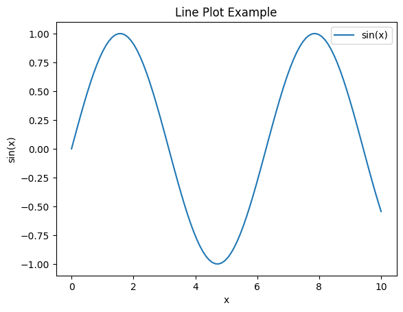
# Example 1: Line plot
x = np.linspace(0, 10, 100)
y = np.sin(x)

plt.figure()
plt.plot(x, y, label='sin(x)')
plt.xlabel('x')
plt.ylabel('sin(x)')
plt.title('Line Plot Example')
plt.legend()
plt.show()

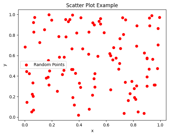
# Example 2: Scatter plot
x = np.random.rand(100)
y = np.random.rand(100)

plt.figure()
plt.scatter(x, y, color='r', label='Random Points')
plt.xlabel('x')
plt.ylabel('y')
plt.title('Scatter Plot Example')
plt.legend()
plt.show()

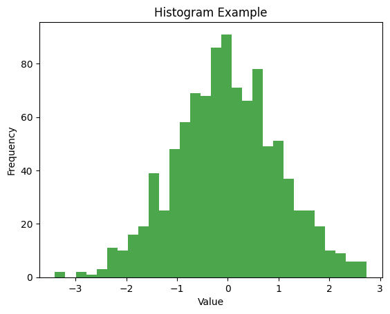
# Example 3: Histogram
data = np.random.randn(1000)

plt.figure()
plt.hist(data, bins=30, alpha=0.7, color='g')
plt.xlabel('Value')
plt.ylabel('Frequency')
plt.title('Histogram Example')
plt.show()

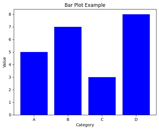
# Example 4: Bar plot
categories = ['A', 'B', 'C', 'D']
values = [5, 7, 3, 8]

plt.figure()
plt.bar(categories, values, color='b')
plt.xlabel('Category')
plt.ylabel('Value')
plt.title('Bar Plot Example')
plt.show()

Materials Informatics

Practical: Setup Programming Environment

Materials Informatics

Computer and Computation