Diffusion Models
Generative models are a class of machine learning techniques designed to learn the underlying distribution of a dataset and generate new samples that resemble the training data. They can be broadly categorized into two types: explicit and implicit generative models. Explicit models, like Gaussian Mixture Models (GMMs), define a probability distribution over the data space, while implicit models, such as Generative Adversarial Networks (GANs) and Diffusion Models, do not explicitly define a distribution but instead learn to generate samples through adversarial training or iterative denoising processes.
Beyond predicting properties of known or hypothetical materials, a grand challenge in materials informatics is inverse design: computationally generating novel material structures that exhibit desired properties. While various generative models exist (like VAEs and GANs), Diffusion Models have recently emerged as a particularly powerful and promising approach, demonstrating the ability to generate high-quality, realistic data in domains like image synthesis, and increasingly, in materials science.
Controlled Corruption and Learned Reversal
Diffusion model framework: forward process (corruption) and reverse process (denoising). Figure adapted from Deep Unsupervised Learning using Nonequilibrium Thermodynamics.
Diffusion models operate based on two complementary processes:
Forward Process (Noise Addition)
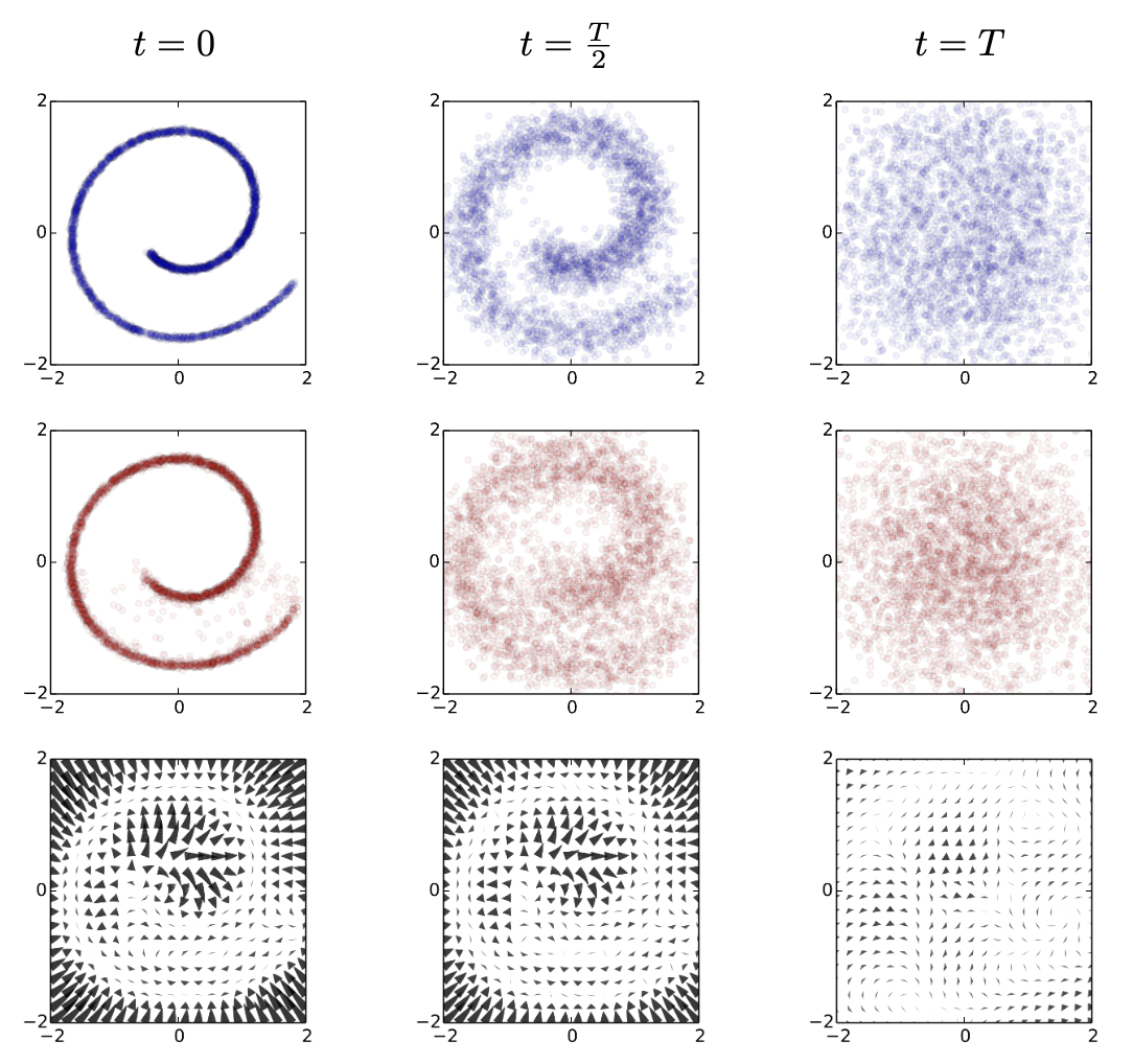
This is a fixed process (no learning involved) where we start with a real data sample (e.g., the atomic coordinates and lattice parameters of a crystal structure). We gradually add a small amount of Gaussian noise over a large number of discrete time steps . If the steps are small enough and is large enough, the distribution at the final step, , becomes indistinguishable from pure Gaussian noise . Mathematically, this defines a sequence of increasingly noisy samples .
Gaussian Noise
Gaussian noise is defined by the equation:
where is the mean and is the variance. It is a common assumption in many physical systems, including atomic structures, where the noise can be thought of as small perturbations to the atomic positions or properties.
At step , we have the original data .
At step , we add a small amount of noise to get
...
At step , we have a sample that is nearly indistinguishable from pure noise.
To formalize this, we define a Markov chain where each step is conditioned on the previous step and a noise term :
where and are predefined noise schedule constants.
Reverse Process (Denoising)
This is where the learning happens. The goal is to learn a “denoiser” model that can reverse the noise addition process. Starting from pure noise , the model iteratively predicts the noise that was added at step (or equivalently, predicts the slightly less noisy sample ) and gradually denoises the sample step-by-step, eventually yielding a generated sample that should resemble the original data distribution.
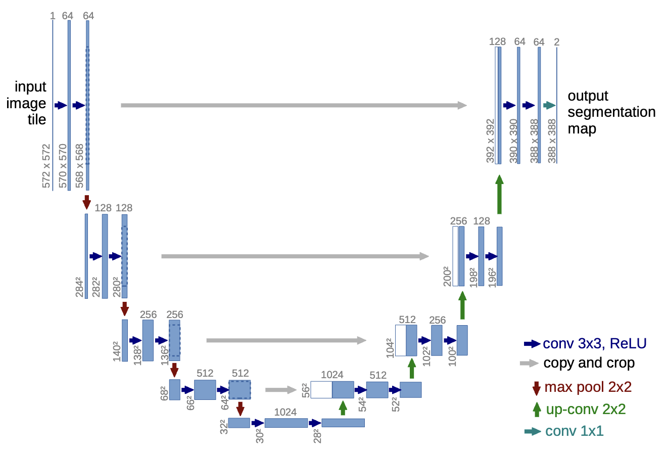
U-Net architecture for denoising. The U-Net consists of an encoder-decoder structure with skip connections, allowing it to capture both local and global features effectively. Figure adapted from U-Net: Convolutional Networks for Biomedical Image Segmentation.
This reverse process is typically parameterized by a neural network (often a U-Net architecture, often incorporating specialized layers like GNNs or equivariant layers when dealing with atomic structures) which is trained to predict the noise added at each step , given the noisy input and the time step .
Generation
Once the denoiser model is trained, we can generate new crystal structures:
Start with Pure Noise: Generate a random sample from the simple noise distribution (e.g., Gaussian noise for coordinates and perhaps random types for atoms initially).
Iterative Denoising: Repeat the following for :
Feed the current noisy structure and the timestep into the trained denoiser model .
Get the model’s prediction of the noise .
Use this predicted noise to calculate an estimate of the previous, slightly less noisy structure . (The exact formula involves and the known noise schedule parameters ).
Final Result: After performing this denoising step times, the resulting should be a novel, realistic crystal structure that follows the patterns learned by the model from the training data.
Analogy: Sculpting from Marble
Think of it like this:
Forward Process: You start with a perfect statue (), grind it down bit by bit (add noise ) until it’s just a formless block of marble dust (, pure noise). This grinding process is simple and predetermined.
Reverse Process (Learning): An AI sculptor learns by looking at countless slightly-ground-down statues () how to predict exactly which bits were ground off () in the last step.
Generation (Sampling): You give the trained AI sculptor a random block of marble dust (). It looks at it, predicts the ‘last bit ground off’, and effectively glues it back on (denoises) to get a slightly more formed block (). It repeats this, using its learned skill at each stage, until it has reconstructed a complete, novel statue ().
Training
The model is trained on many examples of real crystal structures. For each structure, we can simulate the forward process to get noisy versions () and the actual noise () added at each step . The model learns by trying to match its noise prediction to the actual noise, using standard deep learning optimization techniques.
Application to Materials Generation
Applying diffusion models to generate crystal structures presents unique challenges and opportunities:
Data Representation: How do we represent a periodic crystal structure () and add noise to it? Common approaches involve applying noise to fractional atomic coordinates and potentially lattice vectors, while respecting periodic boundary conditions. Ensuring chemical validity (e.g., sensible bond lengths, avoiding atomic clashes) during the denoising process is critical and often requires careful model design or post-processing.
Conditioning: A key advantage of diffusion models is their ability to be conditioned. We can guide the generation process by providing additional information to the denoising network, such as the desired chemical composition, space group, or even target properties (e.g., low formation energy, specific band gap). This allows us to steer the generation towards materials with specific functionalities.
Model Examples: Recent research has introduced models like CDVAE (which uses diffusion in a latent space), DiffCSP, and others specifically designed for generating periodic crystal structures. These models often combine diffusion principles with GNNs or other structure-aware components within the denoising network.
Strengths and Limitations
Strengths:
Capable of generating very high-quality and diverse samples that often capture the data distribution well.
Generally more stable training compared to Generative Adversarial Networks (GANs).
Flexible framework allowing for conditioning on various attributes.
State-of-the-art results in many generative tasks.
Limitations:
Sampling (generation) can be computationally slow as it requires iterating through many denoising steps ( can be large, e.g., 1000).
Relatively new for materials generation; best practices for representing structures and ensuring physical validity are still evolving.
Like other deep learning models, they require significant amounts of training data.
Theoretical understanding is still developing compared to some other generative model classes.